Inter 1st Year

Use these Inter 1st Year Maths 1A Formulas PDF Chapter 6 Trigonometric Ratios up to Transformations to solve questions creatively.

Intermediate 1st Year Maths 1A Trigonometric Ratios up to Transformations Formulas

→ sin θ, cos θ, tan θ, cosec θ, sec θ and cot θ are called circular functions.

→ cosec θ, sec θ and cot θ are reciprocals to sin θ, cos θ and tan θ respectively.

→ sin²θ + cos²θ = 1; 1 + tan²θ = sec²θ; 1 + cot²θ = cosec²θ

→ sec θ + tan θ and sec θ – tan θ are mutual reciprocals.
Similarly cosec θ + cot θ and cosec θ – cot θ are also mutual reciprocals.

→ |sin θ| ≤ 1, |cosec θ| ≥ 1, |cos θ| ≤ 1 and |sec θ| ≥ 1

• sin 0° = o = cos 90°
• sin 15° = \(\frac{\sqrt{3}-1}{2 \sqrt{2}}\) = cos 75°
• sin 18° = \(\frac{\sqrt{5}-1}{4}\) = cos 72°
• sin 30° = \(\frac{1}{2}\) = cos 60°
• sin 36° = \(\frac{\sqrt{10-2 \sqrt{5}}}{4}\) = cos 54°
• sin 45° = \(\frac{1}{\sqrt{2}}\) = cos 45°
• sin 54° = \(\frac{\sqrt{5}+1}{4}\) = cos 36°
• sin 60° = \(\frac{\sqrt{3}}{2}\) = cos 30°
• sin 72° = \(\frac{\sqrt{10+2 \sqrt{5}}}{4}\) = cos 18°
• sin 75° = \(\frac{\sqrt{3}+1}{2 \sqrt{2}}\) = cos 15°
• sin 90° = 1 = cos 0°

Also, tan 15° = 2 – √3, tan 75° = 1 + √3
Sign to the determined by “ALL SILVER CUPS” rules

• sin (90° – θ) = cos θ; sin (90° + θ) = cos θ
• cos (90° – θ) – sin θ; cos (90° + θ) = -sin θ
• sin (180° – θ) = sin θ; sin (1800 + θ)= -sin θ
• cos (180° – θ) = -cos θ; cos (180° + θ) = -cos θ
• sin (270° – θ) = -cos θ; sin (270° + θ) = -cos θ
• cos (270° – θ) = -sin θ; cos (270° + θ) = sin θ
  sin (360° – θ) = -sin θ; sin (360° + θ) = sin θ
• cos (360° – θ) = cos θ; cos (360° + θ) = cos θ When ‘n’ is a +ve integer,
• sin (n. 360° – θ) = -sin θ; sin (n. 360° + θ) = +sin θ
• cos (n. 360° – θ) = cos θ; cos (n. 360° + θ) = cos θ
• sin (-θ) = – sin θ, cos (-θ) = cos 0; tan (-θ) = -tan θ.

→ For 0°, 180°, 360° ……………….. (multplies of π), there is no change in the ratios.

→ For 90°, 270°, 450°…………. (odd multiplies of \(\frac{\pi}{2}\) we get change in the ratio.

• For sin we get cos
• For tan we get cot
• For sec we get cosec
• For cos we get sin
• For cot we get tan
• For cot we get sin

→ Any non-constant function f : R → R is said to be “Periodic”, if there exists a real number p(≠ 0) such that f(x + p) = f(x) for each x ∈ R. The least positive value of ‘p’ with this property is called the “Period” of ‘f’.

→ If ‘f’ is a periodic function with period ‘P’ then

• – f is also a periodic function with period ‘P.
• f(x – p) = f(x), f(x + pn) = f(x) ∀ n ∈ Z, x ∈ R.

→ If f(x) is a periodic function with period ‘P, then f(ax + b) is also a periodic function with period \(\frac{P}{|a|}\)

→ If y = f(x), y = g(x) are periodic functions with l, m as the periods respectively, then a, b ∈ R the function h(x) = af(x) + bg(x) is a period function and L.C.M. of {l, m}
(if exist) is a period of h.

→ \(\frac{2 \pi}{k}\) is the period of sin x, cosec x, cos x and sec x.

→ \(\frac{\pi}{k}\) is the period of tan x and cot x.

→ Range of a sin x + b cos x is \(\left[-\sqrt{a^{2}+b^{2}}, \sqrt{a^{2}+b^{2}}\right]\)

→ Range of a sin x + b cos x + c is [c – \(\sqrt{a^{2}+b^{2}}\), c + \(\sqrt{a^{2}+b^{2}}\)]

→ sin x and cos x are continuous on ‘R’

→ tan x is. discontinuous at x = (2n + 1).\(\frac{\pi}{2}\),n ∈ Z.

→ cot x is discontinuous at x = nπ, n ∈ Z.

→ sec x is discontinuous at x = (2n + 1).\(\frac{\pi}{2}\), n ∈ Z.

→ cosecx is discontinuous at x = nπ, n ∈ Z.

→ sin (A ± B) = sin A cos B ± cos A sin B

→ cos (A ± B) = cos A cos B + sin A sin B

→ tan (A ± B) = \(\frac{\tan A \pm \tan B}{1 \mp \tan A \tan B}\)

→ cot (A ± B) = \(\frac{\cot A \cot B \mp 1}{\cot B \pm \cot A}\)

→ sin (A + B). sin (A-B) = sin²A – sin²B = cos²B – cos²A

→ cos (A + B). cos (A – B) = cos²A – sin²B = cos²B – sin²A

→ sin (A + B + C) = sin A cos B cos C + cos A sin B cos C + cos A cos B sin C – sin A sin B sin C

→ cos (A + B + C) = cos A cos B cos C – cos A sin B sin C – sin A cos B sin C – sin A sin B cos C

→ tan (A + B + C) = \(\frac{\sum \tan A-\pi \tan A}{1-\sum \tan A \tan B}\)

→ sin 2A = 2 sin A cos A, sin A = 2 sin \(\frac{A}{2}\) cos \(\frac{A}{2}\)

→ cos 2A = cos²A – sin²A = 1 – 2 sin² A = 2 cos²A – 1

→ cos A = cos²\(\frac{A}{2}\) sin²\(\frac{A}{2}\) = 1 – 2 sin²\(\frac{A}{2}\) = 2 cos² \(\frac{A}{2}\) – 1

→ tan 2A = \(\frac{2 \tan A}{1-\tan ^{2} A}\), tan A = \(\frac{2 \tan \frac{A}{2}}{1-\tan ^{2} \frac{A}{2}}\)(\(\frac{A}{2}\), A are not odd multiples of \(\frac{\pi}{2}\))

→ cot 2A = \(\frac{\cot ^{2} A-1}{2 \cot A}\), cot A = \(\frac{\cot ^{2} \frac{A}{2}-1}{2 \cot \frac{A}{2}}\); (A is not an integral multiple of π)

→ sin 2A = \(\frac{2 \tan A}{1+\tan ^{2} A}\), sin A = \(\frac{2 \tan \frac{A}{2}}{1+\tan ^{2} \frac{A}{2}}\); (\(\frac{A}{2}\), is not an odd multiple of \(\frac{\pi}{2}\))

→ cos 2A = \(\frac{1-\tan ^{2} A}{1+\tan ^{2} A}\), cos A = \(\frac{1-\tan ^{2} \frac{A}{2}}{1+\tan ^{2} \frac{A}{2}}\)

→ sin 3A = 3sin A – 4 sin³A

→ cos 3A = 4cos³A – 3 cos A

→ tan 3A = \(\frac{3 \tan A-\tan ^{3} A}{1-3 \tan ^{2} A}\)

→ cot 3A = \(\frac{3 \cot A-\cot ^{3} A}{1-3 \cot ^{2} A}\)

→ sin(A + B) + sin (A – B) = 2sin A cos B

→ sin(A + B) – sin(A – B) = 2cos A sin B

→ cos (A + B) + cos (A – B) = 2cos A cos B

→ cos(A + B) – cos(A – B) = -2sin A sin B

→ sin C + sin D = 2sin \(\frac{C+D}{2}\) cos \(\frac{C-D}{2}\)

→ sin C – sin D = 2cos \(\frac{C+D}{2}\) sin \(\frac{C-D}{2}\)

→ cos C + cos D = 2 cos \(\frac{C+D}{2}\) cos \(\frac{C-D}{2}\)

→ cos C – cos D = -2 sin \(\frac{C+D}{2}\) sin \(\frac{C-D}{2}\)

→ For any A ∈ R
(a) sin A = ±\(\sqrt{\frac{1-\cos 2 A}{2}}\)
(b) cos A = ±\(\sqrt{\frac{1+\cos 2 A}{2}}\)
(c) IfA ¡s not an odd multiple of \(\frac{\pi}{2}\), then tan A = ±\(\sqrt{\frac{1-\cos 2 A}{1+\cos 2 A}}\)

→ sin \(\frac{A}{2}=\pm \sqrt{\frac{1-\cos A}{2}}\)

→ cos \(\frac{A}{2}=\pm \sqrt{\frac{1+\cos A}{2}}\)

→ If A is not an odd multiple of n, then tan \(\frac{A}{2}=\pm \sqrt{\frac{1-\cos A}{1+\cos A}}\)

→ If a ray \(\overrightarrow{\mathrm{OP}}\) makes an angle θ with the positive direction of X-axis then

• Sin θ = \(\frac{\mathrm{y}}{\mathrm{r}}\)
• cos θ = \(\frac{\mathrm{x}}{\mathrm{r}}\)
• tan θ = \(\frac{\mathrm{y}}{\mathrm{x}}\) (x ≠ 0)
• cot θ = \(\frac{\mathrm{x}}{\mathrm{y}}\) (y ≠ 0)
• sec θ = \(\frac{\mathrm{r}}{\mathrm{x}}\)(x ≠ 0)
• cosec θ = \(\frac{\mathrm{r}}{\mathrm{y}}\)(y ≠ 0)

Relations :

• sin θ cosec θ = 1
• cos θ sec θ = 1
• tan θ cot θ = 1
• sin² θ + cos² θ = 1
• 1 + tan²θ = sec² θ → (sec θ + tan θ)(sec θ – tan θ) = 1
  → sec θ + tan θ = \(\frac{1}{\sec \theta-\tan \theta}\) = 1
• 1 + cot²θ = cosec²θ → (cosec θ + cot θ) (cosec θ – cot θ) = 1
• sec²θ + cosec²θ = sec²θ. cosec²θ
• tan²θ – sin²θ = tan²θ . sin²θ;
  cot²θ – cos²θ = cot²θ. cos²θ
• sin²θ + cos⁴θ = 1 – sin²θ cos²θ
  = sin⁴θ + cos²θ
• sin⁴θ + cos⁴θ = 1 – 2sin²θ cos²θ
• sin⁶θ + cos⁶ θ = 1 – 3sin²θ cos²θ
• sin²x + cosec²x ≥ 2
• cos²x + sec² x ≥ 2
• tan² x + cot² x ≥ 2.

Values of trigonometric ratios of certain angles

Signs of Trigonometric ratios :
If lies in I, II, III, IV quadrants then the signs of trigonometric ratios are as follows.

Note :

• 0°, 90°, 180°, 270°. 360°, 450°, etc. are called quadrant angles.
• With “ALL SILVER TEA CUPS” symbol we can remember the signs of trigonometric ratios.

Coterminal angles :
If two angles differ by an integral multiples of 360o then two angles are called coterminal angles.
Thus 30°, 390°, 750°, 330° etc., are coterminal angles.

Complementary Angles :
Two Angles A, B are said to complementary ⇒ A + B = 90°

Supplementary angles :
Two angles A, B are said to be supplementary ⇒ A + B = 180°.

→ sin C + sin D = 2sin\(\frac{\mathrm{C}+\mathrm{D}}{2}\). cos \(\frac{\mathrm{C}-\mathrm{D}}{2}\)

→ sin C – sin D = 2cos\( . sin [latex]\frac{\mathrm{C}-\mathrm{D}}{2}\)

→ cos C + cos D = 2cos \(\frac{\mathrm{C}+\mathrm{D}}{2}\). cos \(\frac{\mathrm{C}-\mathrm{D}}{2}\)

→ cos C – cos D = 2sin\(\frac{\mathrm{C}+\mathrm{D}}{2}\). sin \(\frac{\mathrm{D}-\mathrm{C}}{2}\)

→ 2sin A cos B = sin(A + B) + sin(A – B)

→ 2cos A sin B = sin(A + B) – sin(A – B)

→ 2cos A cos B = cos(A + B) + cos(A – B)

→ 2sin A sin B = cos(A – B) – cos(A + B)
(or)
cos(A – B) – cos(A + B) = 2 sin A sin B.

→ \(\frac{\sin A+\sin B}{\sin A-\sin B}\) = tan\(\left(\frac{A+B}{2}\right)\).

→ If sin A + sin B = x, and cos A + cos B = y. Then

• tan\(\left(\frac{\mathrm{A}+\mathrm{B}}{2}\right)=\frac{\mathrm{x}}{\mathrm{y}}\)
• sin(A + B) = \(\frac{2 x y}{y^{2}+x^{2}}\)
• cos (A + B) = \(\frac{y^{2}-x^{2}}{y^{2}+x^{2}}\)
• tan(A + B) = \(\frac{2 x y}{y^{2}-x^{2}}\)

Use these Inter 1st Year Maths 1A Formulas PDF Chapter 7 Trigonometric Equations Functions to solve questions creatively.

Intermediate 1st Year Maths 1A Trigonometric Equations Formulas

→ If K ∈ [-1, 1], then the principal solution θ of sin θ = K lies in \(\left[\frac{-\pi}{2}, \frac{\pi}{2}\right]\)and the general solution is given by nπ + (-1)ⁿ θ, n ∈ Z

→ If K ∈ [-1, 1], then the principal solution θ of cos θ = K lies in [0, π] and the general solution is given by 2nπ ± 0, n ∈ Z

→ If K ∈ R, then the principal solution θ of tan x = K lies in \(\left(\frac{-\pi}{2}, \frac{\pi}{2}\right)\), and the general solution is given by n\left(\frac{-\pi}{2}, \frac{\pi}{2}\right) ± θ, n ∈ Z

→ sin θ = 0 ⇒ θ = nπ, n is an integer and its principal solution is x = 0

→ cos θ = 0 ⇒ θ = (2n + 1)\(\frac{\pi}{2}\), n is an integer and its principal solution is x = \(\frac{\pi}{2}\)

→ tan θ = 0 ⇒ θ = nπ, n is an integer and its principal solution is x = 0

→ cot θ = 0 ⇒ θ = (2n + 1)\(\frac{\pi}{2}\) n is an integer

→ cosec θ = cosec α ⇒ θ = nπ + (-1)ⁿα, n is an integer

→ sec θ = sec α ⇒ θ = 2nπ ± α, n is an integer

→ cot θ = cot α ⇒ θ = nπ ± α and the principal solution α ∈ (0, π)

→ sin²θ = sin² α ⇒ θ = nπ ± α, wherenever a solution exists.

→ cos²θ = cos² α ⇒ θ = nπ ± α, wherenever a solution exists.

→ tan²θ = tan² α ⇒ θ = nπ ± α, wherenever a solution exists.

→ a cos θ + b sin θ = c, (a, b, c) ∈ R and a² + b² ≠ 0 has a solution, iff c² ≤ a² + b².

Trigonometric Equations:
An equation consisting of the trigonometric functions of a variable angle θ ∈ R is called a trigonometric equation.

→ sin θ = 0 ⇒ θ = nπ, where n ∈ Z.

→ cos θ = 0 ⇒ θ = (2n + 1)\(\), where n ∈ Z.

→ tan θ = 0 ⇒ θ = nπ where π is any integer.

→ The solution of sin θ = k (|k|<1) lying between – \(\frac{\pi}{2}\) and \(\frac{\pi}{2}\) is called the principle solution of the equation.

→ The solution of cos θ = k (|k|<1) lying between 0 and π is called the principal solution of the equation.

→ That solution of tan θ = k, lying between – \(\frac{\pi}{2}\) and \(\frac{\pi}{2}\) is called the principal solution of the equation.

→ The general value of θ satisfying cos θ = k (|k| < 1) is given by θ = 2nπ ± α where n ∈Z.

→ The general value of θ satisfying sin θ = k (|k|< 1) is given by θ = nπ + (-1)ⁿα where n ∈ Z.

→ The general value of θ satisfying tan θ = k is given by θ = nπ + α where n ∈ Z. (in each of the above cases, α is the principal solution).

→ If sin0 = k, tan0 = k are given equations, then the general value of θ is given by θ = 2nπ + α where α is that solution lying between 0 and 2π.

→ The equation a cos θ + b sin θ = c will have no solution or will be inconsistent if |c| > \(\sqrt{a^{2}+b^{2}}\)

→ cos nπ = (-1)ⁿ , sin nπ = 0.

→ If sin²θ = sin²α or cos²θ = cos²α or tan²θ = tan²a, then θ = nπ ± α; n ∈ Z.

Use these Inter 1st Year Maths 1A Formulas PDF Chapter 8 Inverse Trigonometric Functions to solve questions creatively.

Intermediate 1st Year Maths 1A Inverse Trigonometric Functions Formulas

→ If sin θ = x and θ ∈ \(\left[\frac{-\pi}{2}, \frac{\pi}{2}\right]\), then sin^-1(x) = θ,

→ If cos θ x and θ ∈ [0, π], then cos^-1(x) = θ

→ If tan θ = x and θ ∈ \(\left(\frac{-\pi}{2}, \frac{\pi}{2}\right)\). then tan^-1 (y) = θ

→ If cot θ = x and θ ∈ (0, π), then cot^-1(x) = θ.

→ If sec θ = x and θ ∈ [o, \(\frac{\pi}{2}\)) ∪ (\(\frac{\pi}{2}\), π] then sec^-1x = θ.

→ If cosec θ = x and θ ∈ [-\(\frac{\pi}{2}\), 0) ∪ (o, \(\frac{\pi}{2}\)] then cosec^-1x = θ.

→ If x ∈ [-1, 1] – {0}, then sin^-1(x) = cosec^-1\(\left(\frac{1}{x}\right)\)

→ If x ∈ [-1, 1] – {0}, then cos^-1(x) = sec^-1\(\left(\frac{1}{x}\right)\)

→ If x > 0, then tan^-1(x) = cot^-1\(\left(\frac{1}{x}\right)\) and
x < 0, then tan^-1(x) = cot^-1\(\left(\frac{1}{x}\right)\) – π

→ sin^-1 x + cos^-1x = \(\frac{\pi}{2}\) (|x| ≤ 1) i.e., – 1 ≤ x ≤ 1

→ tan^-1x + cot^-1x = \(\frac{\pi}{2}\), for any x ∈ R

→ sec^-1x + cosec^-1x = \(\frac{\pi}{2}\), if (-∞, – 1] ∪ [1, ∞)

Function y = f(x)	Domain (x)	Range (y)
(i) sinh-1 (x)	[-1, 1]	\( \left[\frac{-\pi}{2}, \frac{\pi}{2}\right] \)
(ii) cosh-1 (x)	[1, 1]	[0, π]
(iii) tanh-1 (x)	R	\( \left(\frac{-\pi}{2}, \frac{\pi}{2}\right) \)
(iv) cot-1 (x)	R	(0, π)
(v) sec-1 (x)	(-∞, -1] ∪ [1, ∞)	[0, \( \frac{\pi}{2} \)) ∪ (\( \frac{\pi}{2} \), π]
(vi) cosec-1 (x)	(-∞, -1] ∪ [1, ∞)	[-\( \frac{\pi}{2} \), 0) ∪  (0, \( \frac{\pi}{2} \), π]

→ Principal values:
For sin^-1x, tan^-1x, cot^-1x, cosec^-1x, principal values lies between –\(\frac{\pi}{2}\) and \(\frac{\pi}{2}\)
For cos^-1 x, sec^-1 x, principal values lies between 0 and π.

→ tan^-1x + tan^-1y = tan^-1\(\left(\frac{x+y}{1-x y}\right)\) if (xy < 1), x > 0, y > 0
= \(\frac{\pi}{2}\) if (xy = 1), x > 0, y > 0
= π +tan^-1\(\), if (xy > 1), x > 0, y > 0

→ If x < 0, y < 0 then tan^-1x + tan^-1y = tan^-1\(\left(\frac{x+y}{1-x y}\right)\) if xy > 1
= – \(\frac{\pi}{2}\), if xy < 1
= –\(\frac{\pi}{2}\), if xy = 1

→ If x, y ∈ [0, 1] and x² + y² ≤ 1, then sin^-1 x + sin^-1 y = sin^-1\(\left(x \sqrt{1-y^{2}}+y \sqrt{1-x^{2}}\right)\)

→ If x, y ∈ [0, 1] and x² + y² > 1 then sin^-1 x + sin^-1 (y) = π – sin^-1\(\left(x \sqrt{1-y^{2}}+y \sqrt{1-x^{2}}\right)\)

→ If x, y ∈ [0, 1], then sin^-1 x + sin^-1y) = cos^-1(\(\sqrt{1-x^{2}} \sqrt{1-y^{2}}\) – xy)

→ If x, y ∈ [0, 1] then sin^-1 y = sin^-1(x\(\sqrt{1-y^{2}}\) – y\(\sqrt{1-x^{2}}\))

→ If x, y ∈ [0, 1], then cos^-1 x + cos^-1y = cos^-1(\(\sqrt{1-x^{2}} \sqrt{1-y^{2}}\) + xy)

→ If x, y ∈ [0, 1] then cos^-1 x + cos^-1y = cos^-1(xy – \(\sqrt{1-x^{2}} \sqrt{1-y^{2}}\))

→ If x, y ∈ [0, 1] and x² + y² ≥ 1 then cos^-1x + cos^-1y = sin^-1(y\(\sqrt{1-x^{2}}\) + x\(\sqrt{1-y^{2}}\))

→ If 0 ≤ x ≤ y ≤ 1 then cos^-1 x – cos^-1y = cos^-1(xy + \(\sqrt{1-x^{2}} \sqrt{1-y^{2}}\))

→ If x, y ∈ [0, 1], then cos^-1 x – cos^-1y = sin^-1(y\(\sqrt{1-x^{2}}\) – x\(\sqrt{1-y^{2}}\))

→ If x ∈ [-1, 1]- {0}, then sin^-1 (x) = cosec^-1\(\left(\frac{1}{x}\right)\)

→ If x ∈ [-1, 1] – {0}, then cos^-1(x) = sec^-1\(\left(\frac{1}{x}\right)\)

→ If x > 0, then tan^-1x = cot^-1\(\left(\frac{1}{x}\right)\) and

→ If x < 0, then tan^-1x = cot^-1\(\left(\frac{1}{x}\right)\) – π

→ sin^-1(-x) = -sin^-1(x), if x ∈ [-1, 1]

→ cos^-1(-x) = π – cos^-1(x), if x ∈ [-1, 1]

→ tan^-1(-x) = -tan^-1 (x), for any x ∈ R

→ For any x ∈ R, cot-7 (-x) = π – cot^-1(x)

→ If x ∈ [-∞, -1] ∪ [1, ∞) then

• sec^-1(-x) = π – sec^-1(x)
• cosec^-1(-x) = -cosec^-1(x)

→ If θ ∈ \(\left[-\frac{\pi}{2}, \frac{\pi}{2}\right]\), then sin^-1(sin θ) = θ and if x ∈ [-1, 1], then sin(sin^-1x) = x.

→ If θ ∈ [0, π], then cos^-1(cos θ) = θ and if x ∈ [-1, 1], then cos (cos^-1x) = x.

→ If θ ∈ \(\left(-\frac{\pi}{2}, \frac{\pi}{2}\right)\), then tan^-1(tan θ) = θ and for any x ∈ R, then tan(tan^-1x) = x

→ If θ ∈ (0, \(\frac{\pi}{2}\)) ∪ (\(\frac{\pi}{2}\), π) then cot^-1(cot θ) = θ and for any x ∈ R, cot (cot^-1x) = x.

→ If θ ∈ (0, \(\frac{\pi}{2}\)) ∪ (\(\frac{\pi}{2}\), π) then sec^-1(sec θ) = θ and if x ∈ (-∞, -1] ∪ [1, ∞) then sec (sec^-1x) = x.

→ If θ ∈ [-\(\frac{\pi}{2}\), 0) ∪ (0, \(\frac{\pi}{2}\)] then cosec^-1 (cosec θ) = θ and if x ∈ (-∞, -1] ∪ [1, ∞), then cosec (cosec^-1x) = x.

→ θ ∈ [0, π] sin^-1(cos θ) = \(\frac{\pi}{2}\) – θ

→ θ ∈ \(\left[\frac{\pi}{2}, \frac{\pi}{2}\right]\) ⇒ cos^-1(sin θ) = \(\frac{\pi}{2}\) – θ

→ θ ∈ \(\left(-\frac{\pi}{2}, \frac{\pi}{2}\right)\) ⇒ cot^-1(tan θ) = \(\frac{\pi}{2}\) – θ

→ θ ∈ (0, π) ⇒ tan^-1(cot θ) = \(\frac{\pi}{2}\) – θ

→ θ ∈ [-\(\frac{\pi}{2}\), 0) ∪ (0, \(\frac{\pi}{2}\)] ⇒ sec^-1(cosec θ) = \(\frac{\pi}{2}\) – θ

→ θ ∈ [0, \(\frac{\pi}{2}\)) ∪ (\(\frac{\pi}{2}\), π] ⇒ cosec^-1(sec θ) = \(\frac{\pi}{2}\) – θ

→ 0 ≤ x ≤ 1 ⇒ sin^-1(x) = cos^-1\(\left(\sqrt{1-x^{2}}\right)\) and

→ If -1 ≤ x < 0 ⇒ sin^-1(x) = -cos^-1\(\left(\sqrt{1-x^{2}}\right)\)

→ -1 < x < 1 ⇒ sin^-1(x) = tan^-1\(\left(\frac{x}{\sqrt{1-x^{2}}}\right)\)

→ -1 ≤ x < 0 ⇒ cos^-1(x) = π – sin^-1\(\left(\sqrt{1-x^{2}}\right)\) = π + tan^-1\(\left(\frac{\sqrt{1-x^{2}}}{x}\right)\)

→ 0 ≤ x ≤ 7 ⇒ cos^-1(x) = sin^-1\(\left(\sqrt{1-x^{2}}\right)\) = tan^-1\(\left(\frac{\sqrt{1-x^{2}}}{x}\right)\)

→ x > 0 ⇒ tan^-1(x) = sin^-1\(\left(\frac{x}{\sqrt{1+x^{2}}}\right)\) = cos^-1\(\left(\frac{1}{\sqrt{1+x^{2}}}\right)\)

→ tan^-1(x) + tan^-1(y) + tan^-1(z) = tan^-1\(\left[\frac{x+y+z-x y z}{1-x y-y z-z x}\right]\), ifx, y, z have the same sign and xy + yz + zx < 1.

→ 2 sin^-1(x) = sin^-12x\(\sqrt{1-x^{2}}\), if x ≤ \(\frac{1}{\sqrt{2}}\)
= π – sin^-12x\(\sqrt{1-x^{2}}\), if x > \(\frac{1}{\sqrt{2}}\)

→ 2 cos^-1(x) = cos^-1(2x² – 1), if x ≥ \(\frac{1}{\sqrt{2}}\)
= π – cos^-1(1 – 2x²), if x < \(\frac{1}{\sqrt{2}}\)

→ 2 tan^-1(x) = tan^-1\(\left(\frac{2 x}{1-x^{2}}\right)\), if |x| < 1
= π – tan^-1\(\left(\frac{2 x}{1-x^{2}}\right)\), if |x| ≥ 1

→ 2tan^-1(x) = sin^-1\(\left(\frac{2 x}{1+x^{2}}\right)\), ∀ x ∈ R
= cos^-1\(\left(\frac{1-x^{2}}{1+x^{2}}\right)\), if x ≥ 0
= -cos^-1\(\left(\frac{1-x^{2}}{1+x^{2}}\right)\), if x < 0
= tan^-1\(\left(\frac{2 x}{1-x^{2}}\right)\), ∀ x ∈ R

→ 3 sin^-1(x) = sin^-1(3x – 4x³) for 0 ≤ x < \(\frac{1}{2}\)
3 cos^-1(x) = cos^-1(4x³ – 3x) for \(\frac{\sqrt{3}}{2}\) ≤ x < 1
3 tan^-1(x) = tan^-1\(\left\{\frac{3 x-x^{3}}{1-3 x^{2}}\right\}\) for 0 ≤ x < \(\frac{1}{\sqrt{3}}\)

→ If sin θ = x, we write θ = sin^-1x.

→ sin(sin^-1x) = x, sin^-1(sin θ) = θ if ‘θ‘ ∈ \(\left[-\frac{\pi}{2}, \frac{\pi}{2}\right]\)

→ cos(cos^-1x)=x, cos^-1(cos θ) = θ if θ ∈ [0, n]

→ tan (tan^-1x) = x, tan^-1(tan θ) = θ if θ ∈ \(\left(-\frac{\pi}{2}, \frac{\pi}{2}\right)\)

→ That value of sin^-1x lying between – \(\frac{\pi}{2}\) and\(\frac{\pi}{2}\) is called the principal value of sin^-1x.

→ That value of cos^-1x lying between 0 and π is called the principal value of cos^-1x.

→ That value of tan^-1x lying between – \(\frac{\pi}{2}\) and \(\frac{\pi}{2}\) is called the principal value of tan^-1x.

→ If -1 ≤ x ≤ 1, then

• sin^-1(- x) = – sin^-1x
• cos^-1(-x) = π – cos^-1x

→ If x ∈ R , then

• tan^-1(-x) = -tan^-1x
• cot^-1(-x) = π – cot^-1x

→ If x ≤ -1 or x ≥ 1, then

• cosec^-1(-x) = -cosec^-1x
• sec^-1(-x) = π – sec^-1x

→ cosec^-1x = sin^-1\(\frac{1}{x}\) (if x ≠ 0)

→ sec^-1x = cos^-1\(\frac{1}{x}\) (if x ≠ 0)

→ cot^-1x = tan^-1\(\frac{1}{x}\) (if x > 0)
= π + tan^-1\(\frac{1}{x}\) (if x < 0)

→ sin^-1x + cos^-1x = π/2 ,

→ tan^-1x + cot^-1x = π/2,

→ sec^-1x + cosec^-1x = π/2.

→ If sin^-1x + sin^-1y = π/2, then x² + y² = 1.

→ sin(cos^-1x) = \(\sqrt{1-x^{2}}\), cos(sin^-1x) = \(\sqrt{1-x^{2}}\)

→ sin^-1 = cos^-1\(\sqrt{1-x^{2}}\) for 0 ≤ x ≤ 1
= -cos^-1\(\sqrt{1-x^{2}}\) for – 1 ≤ x ≤ 0

Use these Inter 1st Year Maths 1A Formulas PDF Chapter 9 Hyperbolic Functions to solve questions creatively.

Intermediate 1st Year Maths 1A Hyperbolic Functions Formulas

→ e^x = 1 + \(\frac{x}{1 !}+\frac{x^{2}}{2 !}+\frac{x^{3}}{3 !}+\ldots+\frac{x^{n}}{n !}\)+ … ∞

→ sinhx = \(\frac{e^{x}-e^{-x}}{2}\)
and coshx = \(\frac{e^{x}+e^{-x}}{2}\)

→ tanh x = \(\frac{\sinh x}{\cosh x}\),

→ coth x = \(\frac{1}{\tanh x}\),

→ sech x = \(\frac{1}{\cosh x}\)

→ cosech x = \(\frac{1}{\sinh x}\), if x ≠ 0

→ cosh²x – sinh²x – 1, sech²x – 1 – tanh²x, cosech²x = coth²x – 1

Function y = f(x)	Domain (x)	Range (y)
sinh x	R	R
cosh x	R	(1, ∞)
tanh x	R	(1, 1)
coth x	R- {0}	(-∞, -1) ∪ (1, ∞)
sech x	R	(0, 1]
cosech x	R – {0}	R – {0}

→ sinh^-1x = loge [x + \(\sqrt{x^{2}+1}\) ] for all x ∈ R

→ cosh^-1x = loge [x + \(\sqrt{x^{2}-1}\)] for all x ∈ (1, ∞)

→ tanh^-1x = \(\frac{1}{2}\)log_e\(\left(\frac{1+x}{1-x}\right)\), |x| < 1 (i.e) for all x ∈ (-1, -1)

→ coth^-1x = \(\frac{1}{2}\)log_e\(\left(\frac{1+x}{1-x}\right)\), |x| > 1 (i.e) for all x ∈ (-∞, -1) (1, ∞)

→ sech^-1x = log_e\(\left(\frac{1+\sqrt{1+x^{2}}}{x}\right)\) for all x ∈ (0, 1)

→ cosech^-1x = log_e\(\left(\frac{1-\sqrt{1+x^{2}}}{x}\right)\), if x < 0 (i.e,) x ∈ (-∞, 0) and
= log_e\(\left(\frac{1+\sqrt{1+x^{2}}}{x}\right)\), if x > 0 (i.e,) x ∈ (0, ∞)

→ sinh (x + y) = sinh x cosh y + cosh x sinh y

→ cosh (x + y)= cosh x cosh y + sinh x sinh y

→ sinh (x – y) = sinh x cosh y – cosh x sinh y

→ cosh (x – y) = cosh x cosh y – sinh x sinh y

→ tanh (x + y) = \(\frac{\tanh x+\tanh y}{1+\tanh x \tanh y}\)

→ tanh (x – y) = \(\frac{\tanh x-\tanh y}{1-\tanh x \tanh y}\)

→ sinh 2x = 2 sinh x cosh x = \(\frac{2 \tanh x}{1-\tanh ^{2} x}\)

→ cosh 2x = cosh²x + sinh²x
= 2 cosh²x – 1 = 1 + 2 sinh² x = \(\frac{1+\tanh ^{2} x}{1-\tanh ^{2} x}\)

→ tanh 2x = \(\frac{2 \tanh x}{1+\tanh ^{2} x}\)

→ sinh 3x = 3sinh x + 4sinh³ x

→ cosh 3x = 4cosh³ x – 3cosh x

→ tanh 3x = \frac{3 \tanh x+\tanh ^{3} x}{1+3 \tanh ^{2} x}

→ Inverse hyperbolic functions:

Function y = f(x)	Domain (x)	Range (y)
(i) sinh-1(x)	IR	IR
(ii) cosh-1(x)	[1, ∞)	[0, ∞)
(iii) tanh-1(x)	(-1, 1)	IR
(iv) coth-1(x)	R –[-1, 1]	R- {0}
(v) sech-1(x)	(0, 1]	[0, ∞)
(vi) cosech-1(x)	R- {0}	R – {0}

→ sin hx = \(\frac{e^{x}-e^{-x}}{2}\)

→ cos hx = \(\frac{e^{x}+e^{-x}}{2}\)

→ tan hx = \(\frac{e^{x}-e^{-x}}{e^{x}+e^{-x}}\)

→ cosec hx = \(\frac{2}{e^{x}-e^{-x}}\)

→ sec hx = \(\frac{2}{e^{x}+e^{-x}}\)

→ cot hx = \(\frac{e^{x}+e^{-x}}{e^{x}-e^{-x}}\)

→ cos h²x – sinh²x = 1

→ 1 – tanh²x = sech²x

→ cot h²x – 1 = cosech²x

→ Prove that sinh^-1x = log{x + \(\sqrt{x^{2}+1}\)}
Proof:
Let sinh^-1x = y ⇒ x = sinh y

→ Prove that cosh^-1x = log_e(x – \(\sqrt{x^{2}-1}\)
proof:
Let cosh^-1x = y ⇒ x = cosh y

→ Prove that Tan^-1x = \(\frac{1}{2}\)log_e\(\left(\frac{4 x}{1-x}\right)\)
proof:
Let tanh^-1x = y ⇒ x = tanh y

→ sech^-1x = log\(\left\{\frac{1+\sqrt{1-x^{2}}}{x}\right\}\)

→ cosech^-1x = log\(\left(\frac{1-\sqrt{1+x^{2}}}{x}\right)\) x < 0 = log\(\left\{\frac{1-\sqrt{1+x^{2}}}{x}\right\}\) x > 0

→ sin h(x + y) = sin hx cos hy + cos hx sin hy

→ sinh(x – y) = sin hx cos hy + cos hx sin hy

→ cosh(x + y) = cos hx cos hy + sin hx sin hv

→ cosh(x – y) = cos hx cos hy – sin hx sin hy

→ sin h2x = 2 sin hx cos hx = \(\)

→ cos h2x = cosh²x + sinh²x = 2cosh²x – 1 = 1 + 2sinh²x = \(\frac{1+{Tanh}^{2} x}{1-{Tanh}^{2} x}\)

→ Tanh(x + y) = \(\frac{\text { Tanhx+Tanhy }}{1-\text { TanhxTanhy }}\)

→ Tanh(x – y) = \(\frac{\text { Tanhx-Tanhy }}{1+\text { TanhxTanhy }}\)

→ coth(x + y) = \(\frac{\cot h x \cot h y+1}{\cot h y+\cot h x}\)

→ coth(x – y) = \(\frac{\cot h x \cot h y-1}{\cot h y-\cot h x}\)

→ Tanh2x = \(\frac{2 \tan h x}{1+\tanh ^{2} x}\)

→ cot h2x = \(\frac{\operatorname{coth}^{2} x+1}{2 \cot h x}\)

Use these Inter 1st Year Maths 1A Formulas PDF Chapter 4 Addition of Vectors to solve questions creatively.

Intermediate 1st Year Maths 1A Addition of Vectors Formulas

Scalar :
A physical quantity which has only magnitude is called a scalar quantity. All the real numbers will be taken as scalars.

Vector :
A physical quantity which has both magnitude and direction.
e.g. : Velocity acceleration, force, momentum.

Position vector :
Let ‘O’ and ‘P be any points in space. Then OP is called the position vector of the point ‘P w.r.t. origin ‘O’.
Note : \(\overline{A B}\) = Position vector of B- position vector of A’
= \(\overline{O B}-\overline{O A}\)

Coinitial vector:
Vectors having the same initial point are called coinitial vectors.
e.g. : \(\overline{O A}, \overline{O B}, \overline{O C}\) etc.

Unit vector:
A vector whose magnitude is one-unit is called unit vector.
Unit vector in the direction of a is denoted by â = \(\frac{\bar{a}}{|a|}\).
For any non-zero vector \(\bar{a}=|\bar{a}|\) â.

Like vectors :
If two vectors are parallel and having the same direction then they are called like vectors.

Unlike vectors :
If two vectors are parallel and having Opposite direction then they are called unlike vectors.
The position vector of any point C on \(\overline{A B}\) can be taken as λ\(\bar{a}\) + µ\(\bar{a}\), where λ + µ = 1

Angle between vectors:
Let \(\overline{O A}=\bar{a}\) = a, \(\overline{O B}=\bar{a}\) = b be any two non – zero vectors, then angle AOB is defined as angle between vectors \(\bar{a}, \bar{b}\) and is denoted by \((\bar{a}, \bar{b})\) where 0 ≤ \((\bar{a}, \bar{b})\) ≤ 180°.

Addition of vectors (or) Parallelogram Law:
If \(\bar{a}, \bar{b}\) are the adjacent sides of a parallelogram the diagonals which is coinitial with \(\bar{a}, \bar{b}\) is given by \(\bar{a}+ \bar{b}\) and its magnitude is given by
\(|\bar{a}+\bar{b}|=\sqrt{|\bar{a}|^{2}+|\bar{b}|^{2}+2|\bar{a}||\bar{b}| \cos (\bar{a}, \bar{b})}\)

Triangle law:
If two vectors are represented in magnitude and direction by the two sides of a triangle taken in the same order, then their sum is represented by the third side taken in the reverse order.

Note : Addition of vectors is of 2 types :

1. Commutative
2. Associative.

(ie) (i) \(\bar{a}+\bar{b}=\bar{b}+\bar{a}\) and (ii) \((\bar{a}+\bar{b})+\bar{c}=\bar{a}+(\bar{b}+\bar{c})\)
Rule: \(|\bar{a}| \sim|\bar{b}| \leq|\bar{a}-\bar{b}| \leq|\bar{a}+\bar{b}| \leq|\bar{a}|+|\bar{b}|\)

Parallel (or) Collinear vector:

1. Two vectors a, b are parallel or collinear, then a = λ. b, where ‘λ’ is a scalar.
2. If \(\bar{a}\) = (a₁, a₂, a₃), b = (b₁, b₂, b₃) are parallel or collinear, then
   \(\frac{a_{1}}{b_{1}}=\frac{a_{2}}{b_{2}}=\frac{a_{3}}{b_{3}}\)
   Note : Zero vector is parallel to any vector.
3. If three points with position vectors a, b, c are to be collinear. The necessary and sufficient condition is that there exists scalars \(\bar{a}, \bar{b}, \bar{c}\) not all zero, such that
   l\(\bar{a}\) + m\(\bar{b}\) + n\(\bar{c}\) = 0, l + m + n = 0.
4. If \(\bar{a}, \bar{b}, \bar{c}\) are non-zero, non-collinear vectors such that l\(\bar{a}\) + m\(\bar{b}\) + n\(\bar{c}\) = 0, then l = 0, m = 0, n = 0.

Linear combination of vectors :
A linear combination of the system of vectors \(\bar{a}_{1}, \bar{a}_{2}, \ldots, \bar{a}_{n}\) is a vector.
r = x₁\(\bar{a}_{1}\) + x₂\(\bar{a}_{2}\) + x₃\(\bar{a}_{3}\) + ………………. + x_n\(\bar{a}_{n}\)
where x₁ x₂, x₃, ………………., x_n are scalars.

Coplanar vectors:
If three or more vectors lie in the same plane (or) parallel to the same plane then they are called coplanar vectors. If one vector can be expressed as a linear combination of the remaining vectors, then the vectors are coplanar vectors.
If \(\bar{a}\) = x\(\bar{b}\) + y\(\bar{c}\), where x, y, are scalars, then \(\bar{a}, \bar{b}, \bar{c}\) are coplanar.

Linearly dependent system of vectors :
A system of vectors \(\bar{a}_{1}, \bar{a}_{2}, \bar{a}_{3}, \ldots \ldots, \bar{a}_{n}\) is said to
be linearly dependent, if there exists a system of scalars x₁, x₂, x₃, ……………….., x_n not all zero
such that
x₁\(\bar{a}_{1}\) + x₂\(\bar{a}_{2}\) + x₃\(\bar{a}_{3}\) + ………………. + x_n\(\bar{a}_{n}\) = \(\bar{0}\)

• The null vector is linearly dependent.
• Two collinear vectors are linearly dependent.
  \(\bar{a}\) = λ\(\bar{b}\) ⇒ (1)\(\bar{a}\) + (-λ)\(\bar{b}\) = 0
• Any three coplanar vectors are linearly dependent.
  \(\bar{a}\) = x\(\bar{b}\) + y\(\bar{c}\) ⇒ (1)\(\bar{a}\) + (-x)\(\bar{b}\) + (-y)\(\bar{c}\) = 0
• Any four vectors in space from a linearly dependent set of vectors.

Linearly independent system of vectors:
A system of vectors \(\bar{a}_{1}, \bar{a}_{2}, \bar{a}_{3}, \ldots \ldots, \bar{a}_{n}\) is said to be linearly independent, if x₁\(\bar{a}_{1}\) + x₂\(\bar{a}_{2}\) + x₃\(\bar{a}_{3}\) + ………………. + x_n\(\bar{a}_{n}\) = \(\bar{0}\) implies

• Two non-zero, non-collinear vectors are linearly independent.
• Any three non-coplanar vectors are linearly independent. If a, b, c are three non-coplanar vectors and \(\bar{r}\) be any other vector. Then there exists unique scalars x, y, z such that
  \(\bar{r}\) = x\(\bar{a}\) + y\(\bar{b}\) + z\(\bar{c}\).

Right handed system of vectors:
Three non-coplanar vectors \(\bar{a}, \bar{b}, \bar{c}\) are said to form a – right-handed system, if the rotation is form \(\bar{a}\) to \(\bar{b}\) in anti-clockwise direction, through an angle less than 180° as seen from the terminal point of c.
If \(\bar{a}, \bar{b}, \bar{c}\) from RHS and \(\bar{b}, \overline{,}, \bar{a}\) and \(\bar{c}, \bar{a}, \bar{b}\) also from RHS.

Left-handed system of vectors:
Three non-coplanar vectors \(\bar{a}, \bar{b}, \bar{c}\) are said to form a left handed system. If the rotation is from \(\bar{a}\) to \(\bar{b}\) in clockwise direction through an angle less than 180° as seen from terminal point of c.

If \(\bar{a}, \bar{b}, \bar{c}\) are in RHS, then
\(\bar{b}, \overline{,}, \bar{a}\); \(\bar{c}, \bar{a}, \bar{b}\) also from R.H.S.
and \(-\bar{a}, \bar{b}, \bar{c} ; \bar{a},-\bar{b}, \bar{c} ; \bar{a}, \bar{b},-\bar{c}\) form L.H.S.

Direction cosines of a vector and direction ratios of a vector:
If α, β, γ are the angles made by a line with +ve directions of x, y, z axes respectively, then cos α, cos β, cos γ are known as the direction cosines of that line.
Generally the direction cosines are denoted by l, m, n and l² + m² + n² = 1.
Any numbers proportional to the direction cosines are known as direction ratios.

→ Unit vector in the direction of \(\bar{a}\) = \(\frac{\bar{a}}{|\bar{a}|}\)

→ Unit vector parallel to the resultant of the vectors \(\frac{\bar{a}+\bar{b}+\bar{c}}{|\bar{a}+\bar{b}+\bar{c}|}\) is ± \(\frac{\bar{a}+\bar{b}+\bar{c}}{|\bar{a}+\bar{b}+\bar{c}|}\)

→ The vector parallel to the resultant of the vectors \(\frac{\bar{a}+\bar{b}+\bar{c}}{|\bar{a}+\bar{b}+\bar{c}|}\) and having magnitude λ is ±λ \(\frac{\bar{a}+\bar{b}+\bar{c}}{|\bar{a}+\bar{b}+\bar{c}|}\)

→ The position vector of the point which divides the line segment joining the points A and B whose position vectors are \(\bar{a}, \bar{b}\) respectively, internally in the ratio, l:m is \(\frac{m \overline{\mathrm{a}}+l \bar{b}}{l+m}\) externally in the ratio l: m is \(\frac{m \bar{a}-l \bar{b}}{m-l}\), m ≠ l.

→ The ratio in which the line joining the points A(x₁ y₁, z₁) and B(x₂, y₂, z₂) is divided by

• xy – plane is – z₁: z₂
• yz – plane is -x₁ : x₂
• zx – plane is -y₁: y₂

→ If ‘c’ is the mid-point of line AB, the position vector of ‘c’ is \(\overline{O C}=\frac{\overline{O A}+\overline{O B}}{2}\)
= \(\frac{\bar{a}+\bar{b}}{2}\)

→ If \(\bar{a}, \bar{b}\) are two unit vectors, then the unit vector along the bisector of the angle between \(\bar{a}, \bar{b}\) is given by
\(\bar{c}=\frac{\bar{a}+\bar{b}}{|\bar{a}+\bar{b}|}\)
or
\(\bar{c}=\frac{\bar{a}-\bar{b}}{|\bar{a}-\bar{b}|}\)

→ The Vector \(\bar{a}\) = (a₁, a₂, a₃), \(\bar{b}\) = (b₁, b₂, b₃), \(\bar{c}\) = (c₁, c₂, c₃) are coplanar or linearly dependent iff \(\left|\begin{array}{lll}
a_{1} & a_{2} & a_{3} \\
b_{1} & b_{2} & b_{3} \\
c_{1} & c_{2} & c_{3}
\end{array}\right|\) = 0

→ The Vector \(\bar{a}\) = (a₁, a₂, a₃), \(\bar{b}\) = (b₁, b₂, b₃), \(\bar{c}\) = (c₁, c₂, c₃) are non-coplanar or linearly independent iff \(\left|\begin{array}{lll}
a_{1} & a_{2} & a_{3} \\
b_{1} & b_{2} & b_{3} \\
c_{1} & c_{2} & c_{3}
\end{array}\right|\) ≠ 0

→ The necessary and sufficient condition for four points with position vectors \(\bar{a}, \bar{b}, \bar{c}, \bar{d}\) are coplanar is that there exists scalars l, m, n, p not all zero such that
l\(\bar{a}\) + m\(\bar{b}\) + n\(\bar{c}\) + p\(\bar{da}\) = \(\bar{0}\), l + m + n + p = 0.

→ If \(\bar{a}, \bar{b}, \bar{c}\) are three non-zero, non – coplanar vectors and x, y, z are three scalars such that x\(\bar{a}\) + y\(\bar{b}\) + z\(\bar{c}\) = 0, then x = 0, y = 0, z = 0.
Note : Collinearity implies coplanarity but coplanarity does not imply collinearity.

→ If \(\bar{a}\) = (a₁, a₂, a₃), \(\bar{b}\) = (b₁, b₂, b₃), \(\bar{c}\) = (c₁, c₂, c₃) and if \(\left|\begin{array}{lll}
a_{1} & a_{2} & a_{3} \\
b_{1} & b_{2} & b_{3} \\
c_{1} & c_{2} & c_{3}
\end{array}\right|\) > 0 then \(\bar{a}, \bar{b}, \bar{c}\) are in R.H.S

→ If \(\bar{a}\) = (a₁, a₂, a₃), \(\bar{b}\) = (b₁, b₂, b₃), \(\bar{c}\) = (c₁, c₂, c₃) and if \(\left|\begin{array}{lll}
a_{1} & a_{2} & a_{3} \\
b_{1} & b_{2} & b_{3} \\
c_{1} & c_{2} & c_{3}
\end{array}\right|\) < 0 then \(\bar{a}, \bar{b}, \bar{c}\) are in L.H.S

→ If \(\bar{r}\) = x\(\bar{i}\) + y\(\bar{j}\) + z\(\bar{k}\), then |\(\bar{r}\)| = r = \(\sqrt{x^{2}+y^{2}+z^{2}}\) .

→ If l, m, n are the direction cosines of a line, then l² + m² + n² = 1.

→ If a vector makes angles α, β, γ with co-ordinate axes, then

• cos² α + cos² β + cos² γ = 1
• sin² α + sin² β + sin² γ =2

→ The direction ratios of a vector \(\bar{r}\) = a\(\bar{i}\) + b\(\bar{j}\) + c\(\bar{k}\) are a, b, c.

→ If A = (x₁, y₁ z₁), B = (x₂, y₂, z₂) then the direction ratios of a vector
AB are x₂ – x₁, y₂ – y₁, z₂ – z₁

→ If a, b, c are the direction ratios of a vector then direction cosines of a vector are
\(\pm \frac{a}{\sqrt{a^{2}+b^{2}+c^{2}}}, \pm \frac{b}{\sqrt{a^{2}+b^{2}+c^{2}}}, \pm \frac{c}{\sqrt{a^{2}+b^{2}+c^{2}}}\)

→ If a, b, c are the direction ratios of a line then λa, λb, λc also become the direction ratios of that line where ‘λ’ is a non-zero scalar.

→ If \(\bar{r}\) = x\(\bar{i}\) + y\(\bar{j}\) + z\(\bar{k}\), then the direction cosines of a vector are \(\frac{a}{|\vec{r}|}, \frac{b}{|\vec{r}|}, \frac{c}{|\vec{r}|}\)

→ If \(\bar{r}\) = x\(\bar{i}\) + y\(\bar{j}\) + z\(\bar{k}\) makes angles α, γ with co-ordinate axes respectively, then

cos α = \(\frac{a}{|\vec{r}|}\),
cos β = \(\frac{b}{|\vec{r}|}\)
cos γ = \(\frac{c}{|\vec{r}|}\).

• The direction cosines of x- axis are 1, 0, 0.
• The direction cosines of y – axis are 0, 1,0.
• The direction cosines of z- axis are 0, 0, 1.

→ If a vector make equal angles with co-ordinate axes then direction cosines of a vector are \(\pm \frac{1}{\sqrt{3}}, \pm \frac{1}{\sqrt{3}}, \pm \frac{1}{\sqrt{3}}\)

→ If l, m, n are direction cosines of a vector OP and ‘O’ is the origin OP = r, then P = (lr, mr, nr).

→ If 1, m, n are direction cosines of a vector, then the maximum value of lmn is \(\frac{1}{3 \sqrt{3}}\)

→ The maximum value of l + m + n = \(\frac{1}{3 \sqrt{3}}\)

→ The vector equation of a straight-line passing through the point whose position vector is a and parallel to the vector \(\bar{b}\) is \(\bar{r}=\bar{a}+t \bar{b}\), where ‘t’ is parameter.

→ In cartesian form its equation is \(\frac{x-a_{1}}{b_{1}}=\frac{y-a_{2}}{b_{2}}=\frac{z-a_{3}}{b_{3}}\)
where \(\bar{a}\) = (a₁, a₂, a₃), \(\bar{b}\) = (b₁, b₂, b₃).

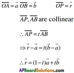
→ The vector equation of a straight-line passing through the point whose position vectors are
a and b is \(\bar{r}\) = (1 – t)\(\bar{a}\) (or) \(\bar{r}=\bar{a}+t(\bar{b}-\bar{a})\); where’t’ is a parameter.

→ In cartesian form \(\frac{x-a_{1}}{b_{1}-a_{1}}=\frac{y-a_{2}}{b_{2}-a_{2}}=\frac{z-a_{3}}{b_{3}-a_{3}}\)
where \(\bar{a}\) = (a₁, a₂, a₃), \(\bar{b}\) = (b₁, b₂, b₃).

→ Vector equation of the plane through the points whose position vectors are \(\bar{a}, \bar{b}, \bar{c}\) is \(\bar{r}=(1-s-t) \bar{a}+s \bar{b}+t \bar{c}\), where s and t are parameters (or)
\(\bar{r}=\bar{a}+s(\bar{b}-\bar{a})+t(\bar{c}-\bar{a})\).
where \(\bar{a}\) = (a₁, a₂, a₃), \(\bar{b}\) = (b₁, b₂, b₃), \(\bar{c}\) = (c₁, c₂, c₃)

→ The vector equation of the plane through the point whose position vector is \(\bar{a}\) and parallel to the vectors \(\bar{b}\) and \(\bar{c}\) is \(\bar{r}=\bar{a}+s \bar{b}+t \bar{c}\), where ‘s’ and ‘t’ are parameter.
In cartesian form it is \(\left|\begin{array}{ccc}
x-a_{1} & y-a_{2} & z-a_{3} \\
b_{1} & b_{2} & b_{3} \\
c_{1} & c_{2} & c_{3}
\end{array}\right|\) = 0

→ Vector equation of the plane through the point’s whose position vectors are a, b and parallel to vector c is
\(\bar{r}=(1-s) \bar{a}+s \bar{b}+t \bar{c}\)
or
\(\bar{r}=\bar{a}+s(\bar{b}-\bar{a})+t \bar{c}\)
In cartesian form it is \(\left|\begin{array}{ccc}
x-a_{1} & y-a_{2} & z-a_{3} \\
b_{1}-a_{1} & b_{2}-a_{2} & b_{3}-a_{3} \\
c_{1} & c_{2} & c_{3}
\end{array}\right|\) = 0

Scalar:
A quantity which has only magnitude but no directions is called scalar quantity.
Ex: Length, mass, time ………….

Vector:
A quantity which has both magnitude and direction is called a vector quantity
Ex: Displacement, Velocity, Force ………………
A vector can also be denoted by a single letter \(\vec{a}, \vec{b}, \vec{c}\) …….. or bold letter a, b, c
Length of \(\vec{a}\) is dinded by |\(\vec{a}\)|. Length of \(\vec{a}\) is called magnitude of \(\vec{a}\).

Zero vector (Null Vector):
The vector of length O and having any direction is called null vector. It is denoted by \(\bar{O}\)

Note:

• If A is any point in the space then \(\overrightarrow{A A}=\vec{O}\)
• A non zero vector is called a proper vector.

Free vector:
A vector which is independent of its position is called free vector

Localised vector:
If \(\vec{a}\) is a vector P is a point then the ordere of pair, (P,a) is called localized vector at P

Multiplication of a vector by a scalar:

• Let m be any scalar and \(\vec{a}\) be any vector then the vector m \(\vec{a}\) is defined as
• Length of m \(\vec{a}\) is |m| times of length of \(\vec{a}\) i.e. |m\(\vec{a}\)| = |m||a|
• The line of support of m\(\vec{a}\) is same or parallel to that of \(\vec{a}\)

The sense the direction of m\(\vec{a}\) is same as that of \(\vec{a}\) if m is positive, the direction of m\(\vec{a}\) is opposite to that \(\vec{a}\) if m is negative

Note:

• o\(\vec{a}\) = o
• m\(\vec{0}\) = \(\vec{0}\)
• (mn)\(\vec{a}\) = m(n\(\vec{a}\)) = n(m\(\vec{a}\))
• (-1)\(\vec{a}\)

Negative of a vector:
\(\vec{a}\) ,\(\vec{b}\) are two vectors having same length but their directions are opposite to each other then each vector is called the negative of the other vector.
Here \(\vec{a}\) = –\(\vec{b}\) and \(\vec{b}\) = –\(\vec{a}\)

Unit vector:
A vector whose magnitude is unity is called unit vector.
Note: If \(\vec{a}\) is any vector then unit vector is \(\frac{\vec{a}}{|\vec{a}|}\) this is denoted by â {read as ‘a’ cap}

Collinear or parallel vectors:
Two or more vectors are said to the collinear vectors if the have same line of support. The vectors are said to be parallel if they have parallel lines of support.

Like parallel vectors:
Vectors having same direction are called like parallel vectors.

Unlike parallel vectors:
Vectors having different direction are called unlike parallel vectors.

Note:

• If \(\vec{a}\), \(\vec{b}\) are two non-zero collinear or parallel vectors then there exists a non zero scalar m such that \(\vec{a}\) = m\(\vec{b}\)
• Conversly if there exists a relation of the type \(\vec{a}\) = m\(\vec{b}\) between two non zero two non zero vectors a, b then a, b must be parallel or collinear.

Cointialvectors:
The vectors having the same initial point are called co-initial vectors.

Co planar vectors:
Three or more vectors are said to be coplanar if they lie on a plane parallel to same plane. Other wise the vectors are non coplanar vectors.

Angle between two non-zero vectors:
Let \(\overline{O A}=\vec{a}\) and \(\overline{O B}=\vec{b}\) be two non-zero vectors. Then the angle between \(\vec{a}\) and \(\vec{b}\) is defined as that angle AOB where O ≤ ∠AOB ≤ 180°

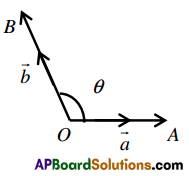
The angle between \(\vec{a}\) and \(\vec{b}\) is denoted by (\(\vec{a}\), \(\vec{b}\))

Note:

• If \(\vec{a}\) and \(\vec{b}\)are any two vectors such that (\(\vec{a}\), \(\vec{b}\)) = 0 then o ≤ 0 ≤ 180° {this is the range of θ i.e. angle beween vectors}
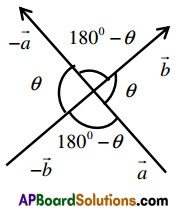
• \((\vec{a}, \vec{b})=(\vec{b}, \vec{a})\)
• \((\vec{a},-\vec{b})=(-\vec{a}, \vec{b})\) = 180° – \((\vec{a}, \vec{b})\)
• \((-\vec{a},-\vec{b})=(\vec{a}, \vec{b})\)

• If k > 0; 1 > 0 then \((k \vec{a}, l \vec{b})=(\vec{a}, \vec{b})\)
• If \((\vec{a}, \vec{b})\) = 0 then \(\vec{a}, \vec{b}\) are like parallel vectors
• If \((\vec{a}, \vec{b})\) = 180° then \(\vec{a}, \vec{b}\) are unlike parallel vectors
• If \((\vec{a}, \vec{b})\) = 90° then \(\vec{a}, \vec{b}\) are orthogonal or perpendicular vectors.

Addition of vectors:
Let \(\vec{a}\) and \(\vec{b}\) be any two given vectors. If three points O, A, B are taken such that \(\overline{O A}=\vec{a}\), \(\overrightarrow{A B}=\vec{b}\) then vectors \(\) is called the vector sum or resultant of the given vectors a and b we write \(\overline{O B}=\overline{O A}+\overline{A B}=\vec{a}+\vec{b}\)

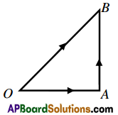
Triangular law of vectors:
Trianglular law states that if two vectors are represented in magnitude and direction by two sides of a triangle taken in order, then their sum or resultant is represented in magnitude and direction by the third side of the triangle taken in opposite direction.

Position vector:
Let O be a fixed point in the space called origin. If P is any point in the space then \(\) is called position vector of P relative to O.

Note:
If \(\vec{a}\) and \(\vec{b}\) be two non collinear vectors, then there exists a unique plane through a,b this plane is called plane generated by a, b. If \(\overline{O A}=\vec{a} ; \overline{O B}=\vec{b}\) then the plane generated by \(\vec{a}\), \(\vec{b}\) is denoted by \(\overline{A O B}\).

• Two non zero vectors a, b are collinear if m\(\vec{a}\) + n\(\vec{b}\) = 0 for some scalars m,n not both zero
• Let \(\vec{a}, \vec{b}, \vec{c}\) be the position vectors of the points A, B, C respectively. Then A, B, C are collinear iff m\(\vec{a}\) + n\(\vec{b}\) + p\(\vec{c}\) = 0 for some scalars m, n, p not all zero such that m + n + p = 0
• Let \(\vec{a}, \vec{b}\) be two non collinear vectors, If \(\vec{r}\) is any vector in the plane generated by a,b then there exist a unique pair of real numbers x, y such that \(\vec{r}\) = x\(\vec{a}\) + y\(\vec{b}\).
• Let \(\vec{a}, \vec{b}\) be two non collinear vectors. If \(\vec{r}\) is any vector such that \(\vec{r}\) = xa + yb for some real numbers then \(\vec{r}\) lies in the plane generated by a, b.
• Three vectors \(\vec{a}, \vec{b}, \vec{c}\) coplanar iff x\(\vec{a}\) + y\(\vec{b}\) + z\(\vec{c}\) = 0 for some scalars x, y, z not all zero.
• Let \(\vec{a}, \vec{b}, \vec{c}, \vec{d}\) be the position vectors of the points A, B, C, D in which no three of them are collinear. Then A, B, C, D are coplanar iff m\(\vec{a}\) + n\(\vec{b}\) + p\(\vec{c}\) + q\(\vec{d}\) = 0 for some scalars m,n,p,q not all zero such that m + n + p + q = 0
• If \(\vec{a}, \vec{b}, \vec{c}\) are three non coplanar vectors and \(\vec{r}\) is any vector then there exist a unique traid of real numbers. x, y, z such that \(\vec{r}\) = x\(\vec{a}\) + y\(\vec{b}\) + z\(\vec{c}\).

Right handed system of orthonormal vectors
A triced of three non-coplanar vectors\(\vec{i}, \vec{j}, \vec{k}\) is said to be a right hand system of orthonormal triad of vectors if

• \(\vec{i}, \vec{j}, \vec{k}\) from a right handed system
• \(\vec{i}, \vec{j}, \vec{k}\) are unit vectors
• (i, j) = 900 = \((\vec{j}, \vec{k})=(\vec{k}, i)\)

Right handed system:
Let \(\overline{O A}=\vec{a}, \overline{O B}=\vec{b}\) and \(\overrightarrow{O C}=\vec{c}\) be three non coplanar vectors. If we observe from the point C that a rotation from OA to OB through an angle not greater than 1800 is in the anti clock wise direction then the vectors a,b, c are said to form ‘Right handed system’.

Left handed system:
If we observe from C that a rotation from OA to OB through an angle not greater than 1800 is in the clock -wise direction then the vectors a,b, c are said to form a “Left handed system”.
If \(\vec{r}=x \vec{i}+y \vec{j}+z \vec{k}\) then \(|\vec{r}|=\sqrt{x_{2}+y_{2}+z_{2}}\).

Direction Cosines:
If a given directed line makes angles α, β, γ, with positive direction of axes of x,y, and z respectively then cos α,cos β,cos γ are called direction cosines of the line and these are denoted by l,m,n.

Direction ratios:
Thre real numbers a,b,c are said to be direction ratios of a line if a:b:c = l:m:n where l,m,n are the direction cosines of the line.

Linear combination:
Let \(\vec{a}_{1}, \bar{a}_{2}, \overline{a_{3}} \ldots \ldots \overline{a_{n}}\) be n vectors and l₁,l₂,l₃….l_n be n scalars then \(l_{1} \bar{a}_{1}+l_{2} \overline{a_{2}}+l_{3} \overline{a_{3}}+\ldots+l_{n} \overline{a_{n}}\) is called a. linear combination of \(\vec{a}_{1}, \bar{a}_{2} \ldots \ldots . \overline{a_{n}}\)

Linear dependent vectors:
The vectors \(\bar{a}_{1}, \overline{a_{2}} \ldots \ldots \overline{a_{n}}\) are said to be linearly dependent if there exist scalars l₁,l₂,l₃….l_n not all zero such that \(_{1} \vec{a}_{1}+l_{2} \overline{a_{2}}+\ldots+l_{n} \overline{a_{n}}]\) = 0

Linear independent The vectors a₁, a₂, a₃ ……………. a_n are said to be linearly independt if l₁, l₂, l₃ ……………. l_n are scalars, \(l_{1} \vec{a}_{1}+l_{2} \overline{a_{2}}+\ldots l_{n} \overline{a_{n}}\) = 0
⇒ l₁ = 0 l₂ = o…. l_n = o

• Let \(\vec{a}, \vec{b}\) be the position vectors of A, B respectively the position vector of the point P which divides \(\overline{A B}\) in the ratio m:n is \(\frac{m \vec{b}+n \vec{a}}{m+n}\). Conversely the point P with position vector \(\frac{m \vec{b}+n \vec{a}}{m+n}\) lies on the lines \(\overline{A B}\) and divides \(\overline{A B}\) in the ratio m:n.
• The medians of a triangle are concurrent. The point of concurrence divides each median in the ratio 2:1
• Let ABC be a triangle and D be a point which is not in the plane of \(\overline{A B C}\) the lines joining O, A, B,C with the centroids of triangle ABC, triangle BCD, triangle CDA and triangle DAB respectively are concurrent and the point of concurrence divides each line segment in the ratio 3:1
• The equation of the line passing through the point A = (x₁, y₁, z₁) and parallel to the vector b = (l, m, n) is \(\frac{x-x_{1}}{l}=\frac{y-y_{1}}{m}=\frac{z-z_{1}}{n}\) = t
• The equation of the line having through the points A(x₁, y₁, z₁), B(x₂, y₂, z₂) is \(\frac{x-x_{1}}{x_{2}-x_{1}}=\frac{y-y_{1}}{y_{2}-y_{1}}=\frac{z-z_{1}}{z_{2}-z_{1}}\) = t
• The unit vector bisecting the angle between the vectors \(\vec{a}, \vec{b}\) is \(\frac{\hat{a}+\hat{b}}{|\hat{a}+\hat{b}|}\)
• The internal bisector the angle between \(\vec{a}, \vec{b}\) is \(\frac{\overline{O P}}{O P}=\frac{\hat{a}+\hat{b}}{|\hat{a}+\hat{b}|}\) are concurrent

Theorem 1:
The vector equation of a line parallel to the vector \(\vec{b}\) and passing through the point A with position vector \(\vec{a}\) is \(\vec{r}=\vec{a}+t \vec{b}\) where t is a scalar.
Proof:
Let \(\overline{O A}=t \vec{a}\) be the given point and \(\overline{O P}=\vec{r}\) be any point on the line
\(\overline{A P}=t \vec{b}\) where ‘t’ is a scalar
\(\vec{r}-\vec{a}=t \vec{b} \Rightarrow \vec{r}=\vec{a}+t \vec{b}\)

Theorem 2:
The vector equation of the line passing through the points A, B whose position vectors \(\vec{a}, \vec{b}\) respectively is \(\vec{r}=\vec{a}(1-t)+t \vec{b}\) where t is a scalar.
Proof:
let P a a point on the line joining of A, B

Theorem 3:
The vector equation of the plane passing through the point A with position vector \(\vec{b}, \vec{c}\) and parallel to the vectors \(\vec{a}\) is \(\vec{r}=\vec{a}+s \vec{b}+t \vec{c}\) where s,t are scalars
Proof:
Given that \(\overline{O A}=\vec{a}\)
Let \(\overline{O P}=\vec{r}\) be the position vector of P
\(\overrightarrow{A P}, \vec{b}, \vec{c}\) are coplanar
∴ \(\overrightarrow{A P}=s \vec{b}+t \vec{c} \Rightarrow \vec{r}-\vec{a}=s \vec{b}+t \vec{c}\)
∴ \(\vec{r}=\vec{a}+s \vec{b}+t \vec{c}\)

Theorem 4:
The vector equation of the plane passing through the points A, B with position vectors \(\vec{a}, \vec{b}\) and parallel to the vector \(\vec{c}\) is \(\vec{r}=(1-s) \vec{a}+s \vec{b}+t \vec{c}\)
Proof:
Let P be a point on the plane and \(\overline{O P}=\vec{r}\)
\(\overline{O A}=\vec{a} \overline{O B}=\vec{b}\) be the given points \(\overline{A P}, \overrightarrow{A B}, \vec{C}\) are coplanar
\(\overrightarrow{A P}=s \overrightarrow{A B}+t \vec{C}\)
\(\vec{r}-\vec{a}=s(\vec{b}-\vec{a})+t \vec{c}\)
\(\vec{r}=(1-s) \vec{a}+s \vec{b}+t \vec{c}\)

Theorem 5:
The vector equation of the plane passing through the points A, B, C having position vectors \(\vec{a}, \vec{b}, \vec{c}\) is \(\vec{r}=(1-s-t) \vec{a}+s \vec{b}+t \vec{c}\) where s,t are scalars
Proof:
Let P be a point on the plane and \(\overline{O P}=\vec{r}\)
\(\overline{O A}=\vec{a} \overline{O B}=\vec{b}, \overline{O C}=\bar{c}\)
Now the vectors \(\overline{A B}, \overline{A C}, \overline{A P}\) are coplanar.
Therefore, \(\overline{A P}=s \overline{A B}+t \overline{A C}\), t,s are scalars.
\(\bar{r}-\bar{a}=s(\bar{b}-\bar{a})+t(\bar{c}-\bar{a})\)
\(\vec{r}=(1-s-t) \vec{a}+s \vec{b}+t \vec{c}\)

Use these Inter 1st Year Maths 1A Formulas PDF Chapter 10 Properties of Triangles to solve questions creatively.

Intermediate 1st Year Maths 1A Properties of Triangles Formulas

→ Sine Rule :
In ΔABC \(\frac{a}{\sin A}=\frac{b}{\sin B}=\frac{c}{\sin C}\) = 2R where R is the circumradius of ΔABC.

→ Cosine Rule :
a² = b² + c² – 2bc. cos A ;
b² = c² + a² – 2ca.cos B;
c² = a² + b² – 2ab. cos C.

→ cos A = \(\frac{b^{2}+c^{2}-a^{2}}{2 b c}\),
cos B = \(\frac{c^{2}+a^{2}-b^{2}}{2 c a}\),
cos C = \(\frac{a^{2}+b^{2}-c^{2}}{2 a b}\)

→ a = b cos C + c cos B,b = c cos A + a cos C and c = a cos B + b cos A (Projection rule)

→ tan \(\frac{B-C}{2}=\frac{b-c}{b+c}\) cot\(\frac{A}{2}\) (Napier’s analogy or tangent rule)

• sin\(\frac{A}{2}\) = \(\sqrt{\frac{(s-b)(s-c)}{b c}}\)
• cos\(\frac{A}{2}\) = \(\sqrt{\frac{s(s-a)}{b c}}\)
• tan\(\frac{A}{2}\) = \(\sqrt{\frac{(s-b)(s-c)}{s(s-a)}}=\frac{\Delta}{s(s-a)}\)

→ Δ = area of ΔABC = \(\frac{1}{2}\) bc sin A = \(\frac{1}{2}\) ca sin B = \(\frac{1}{2}\) ab sin C
= \(\sqrt{s(s-a)(s-b)(s-c)}=\frac{a b c}{4 R}\)
= 2R² sin A sin B sin C

• r = \(\frac{\Delta}{s}\)
• r₁ = \(\frac{\Delta}{s-a}\)
• r₂ = \(\frac{\Delta}{s-b}\)
• r₃ = \(\frac{\Delta}{s-c}\)

→ r = 4 R sin \(\frac{A}{2}\) sin \(\frac{B}{2}\) sin \(\frac{C}{2}\); r₁ = 4Rsin \(\frac{A}{2}\) cos \(\frac{B}{2}\) cos \(\frac{C}{2}\)

→ r = (s – a) tan \(\frac{A}{2}\);
r₁ = s tan \(\frac{A}{2}\) = (s – c) cot \(\frac{B}{2}\) = (s – b) cot \(\frac{C}{2}\)

Mollweide rule:
In ΔABC \(\frac{a+b}{c}=\frac{\cos \left(\frac{A-B}{2}\right)}{\sin \frac{C}{2}}\)
\(\frac{b+c}{a}=\frac{\cos \left(\frac{B-C}{2}\right)}{\sin \frac{A}{2}}\)
\(\frac{c+a}{b}=\frac{\cos \left(\frac{C-A}{2}\right)}{\sin \frac{B}{2}}\)

Sine rule :
In ΔABC, \(\frac{\mathrm{a}}{\sin \mathrm{A}}=\frac{\mathrm{b}}{\sin \mathrm{B}}=\frac{\mathrm{c}}{\sin \mathrm{C}}\) = 2R Where R is the circum – radius.
⇒ a = 2R sin A, b = 2R sin B, c = 2R sin C
a : b : c = sin A : sin B : sin C.

Cosine rule :
In ΔABC,
a² = b² + c² – 2bc cos A
b² = c² + a² – 2ac cos B
c² = a² + b² – 2ab cos C
or
cos A = \(\frac{\mathrm{b}^{2}+\mathrm{c}^{2}-\mathrm{a}^{2}}{2 \mathrm{bc}}\)
cos B = \(\frac{c^{2}+a^{2}-b^{2}}{2 c a}\)
cos C = \(\frac{a^{2}+b^{2}-c^{2}}{2 a b}\) ⇒ cos A : cos B : cos C
= a(b² + c² – a²) : b(c² + a² – b²) : c(a² + b² – c²)

Projection rule :
In ΔABC

• a = b cos C + c cos B,
• b = c cos A + a cos C,
• c = s cos B + b cos A

Mollwiede’s rule :
In ΔABC

• \(\frac{a-b}{c}=\frac{\sin \frac{A-B}{2}}{\cos \frac{C}{2}}\)
• \(\frac{a+b}{c}=\frac{\cos \frac{A-B}{2}}{\sin \frac{C}{2}}\)

Similarly the other two can be written by symmetry.

Tangent rule (or) Napier’s analogy :
In ΔABC

Half angle formulae :

cot A = \(\frac{\mathrm{b}^{2}+\mathrm{c}^{2}-\mathrm{a}^{2}}{4 \Delta}\)
cot B = \(\frac{c^{2}+a^{2}-b^{2}}{4 \Delta}\)
cot C = \(\frac{a^{2}+b^{2}-c^{2}}{4 \Delta}\)

→ Area of ΔABC 1s given by

• Δ = \(\frac{1}{2}\)ab sin C = \(\frac{1}{2}\)bc sin A = \(\frac{1}{2}\) ca sin B
• Δ = \(\sqrt{s(s-a)(s-b)(s-c)}\).
• Δ = \(\frac{a b c}{4 R}\)
• Δ = 2R² sin A sin B sin C
• Δ = rs
• Δ = \(\sqrt{\mathrm{rr}_{1} \mathrm{r}_{2} \mathrm{r}_{3}}\)

→ If ‘r’ is radius of in circle and r₁, r₂, r₃ are the radii of ex-circles opposite to the vertices A, B, C of ΔABC respectively then
i. r = \(\frac{\Delta}{\mathrm{s}}\), r₁ = \(\frac{\Delta}{\mathrm{s-a}}\), r₂ = \(\frac{\Delta}{\mathrm{s-b}}\), r₃ = \(\frac{\Delta}{\mathrm{s-c}}\)

→ r = 4R sin\(\frac{\mathrm{A}}{2}\)sin\(\frac{\mathrm{B}}{2}\) sin\(\frac{\mathrm{C}}{2}\)

• r₁ = 4R sin\(\frac{\mathrm{A}}{2}\)cos\(\frac{\mathrm{B}}{2}\)cos\(\frac{\mathrm{C}}{2}\)
• r₂ = 4R cos\(\frac{\mathrm{A}}{2}\)sin\(\frac{\mathrm{B}}{2}\) cos\(\frac{\mathrm{C}}{2}\)
• r₃ = 4R cos\(\frac{\mathrm{A}}{2}\)cos\(\frac{\mathrm{B}}{2}\) sin\(\frac{\mathrm{C}}{2}\)

→ r = (s – a)tan\(\frac{A}{2}\) = (s – b)tan\(\frac{B}{2}\) = (s – c)tan\(\frac{C}{2}\)

• r₁ = s tan\(\frac{A}{2}\) = (s – b)cot\(\frac{C}{2}\) = (s – c)cot\(\frac{B}{2}\)
• r₂ = s tan\(\frac{B}{2}\) = (s – c)cot\(\frac{A}{2}\) = (s – a)cot\(\frac{c}{2}\)
• r₁ = s tan\(\frac{A}{2}\) = (s – a)cot\(\frac{B}{2}\) = (s – b)cot\(\frac{A}{2}\)

→ \(\frac{1}{r}=\frac{1}{r_{1}}+\frac{1}{r_{2}}+\frac{1}{r_{3}}\)

→ rr₁r₂r₃ = Δ²

→ r₁r₂ + r₂r₃ + r₃r₁ = s²

→ r(r₁ + r₂ + r₃) = ab + bc + ca – s²

→ (r₁ – r)(r₂ + r₃) = a²

→ (r₂ – r)(r₃ + r₁) = b²

→ (r₃ – r)(r₁ + r₂) = c²

→ a = (r₂ + r₃)\(\sqrt{\frac{r r_{1}}{r_{2} r_{3}}}\)

→ b = (r₃ + r₁)\(\sqrt{\frac{r r_{2}}{r_{3} r_{1}}}\)

→ c = (r₁ + r₂)\(\sqrt{\frac{r r_{3}}{r_{1} r_{2}}}\)

→ r₁ – r = 4Rsin²\(\frac{A}{2}\)

→ r₂ – r = 4Rsin²\(\frac{B}{2}\)

→ r₃ – r = 4Rsin²\(\frac{C}{2}\)

→ r₁ + r₂ = 4R cos²\(\frac{C}{2}\)

→ r₂ + r₃ = 4R cos²\(\frac{A}{2}\)

→ r₃ + r₁ = 4R cos²\(\frac{B}{2}\)

→ r₁ + r₂ + r₃ = 4R

→ r + r₂ + r₃ – r₁ = 4R cos A

→ r + r₁ + r₃ – r₂ = 4R cos B

→ r + r₁ + r₂ – r₃ = 4R cos C

→ In an equilateral triangle of side ‘a’
area = \(\frac{\sqrt{3} a^{2}}{4}\)
R = a/√3
r = R/2
r₁ = r₂ + r₃ = 3R/2
r : R : r₁ = 1 : 2 : 3

In circle:
The circle that touches the three sides of a triangle ABC internally is called the “in circle” or inscribed” of its triangle. The centre of the circle is called Incentre denoted by I the radius of the circle is denoted by inradius denoted by Y

→ In a triangle ABC

Excircle:
The circle that touches the side BC (opposite to angle A) internally and the other two sides AB and AC externally is called Excircle. The centre of this circle is called excentre opposite to ‘A’. denoted by I₁. The radius of this circle is called ex-radius, denoted by r₁

|||^ly exradius opposite to angle B is denoted by r₂. The centre of this excircle is denoted by I₂ exradius opposite to angle C is denoted by r₃. The centre of this ex-circle is denoted by I₃

In a triangle ABC

• r₁ = \(\frac{\Delta}{s-a}\)
• r₂ = \(\frac{\Delta}{s-b}\)
• r₃ = \(\frac{\Delta}{s-c}\)

→ r₁ = s tan A/2

→ r₂ = s tan B/2

→ r₂ = s tan C/2

→ r₁ = (s – c)cot\(\frac{B}{2}\)
= (s- b)cot\(\frac{C}{2}\)

→ r₁ = (s – a)cot\(\frac{C}{2}\)
= (s – c)cot\(\frac{A}{2}\)

→ r₁ = (s – a)cot\(\frac{B}{2}\)
= (s – c)cot\(\frac{A}{2}\)

→ r₁ = \(\frac{a}{\tan \frac{B}{2}+\tan \frac{C}{2}}\)

→ r₂ = \(\frac{b}{\tan \frac{C}{2}+\tan \frac{A}{2}}\)

→ r₃ = \(\frac{c}{\tan \frac{A}{2}+\tan \frac{B}{2}}\)

→ r₁ = 4Rsin\(\frac{A}{2}\)cos\(\frac{B}{2}\)cos\(\frac{C}{2}\)

→ r₂ = 4Rcos\(\frac{A}{2}\)sin\(\frac{B}{2}\)cos\(\frac{C}{2}\)

→ r₃ = 4Rcos\(\frac{A}{2}\)cos\(\frac{B}{2}\)sin\(\frac{C}{2}\)

Use these Inter 1st Year Maths 1A Formulas PDF Chapter 3 Matrices to solve questions creatively.

Intermediate 1st Year Maths 1A Matrices Formulas

→ An ordered rectangular array of elements is called a matrix.

→ A matrix in which the number of rows is equal to the number of columns, is called a square matrix. Otherwise it is called rectangular matrix. In a square matrix, an element a_ij is in principal diagonal, if i = j

→ If each non-diagonal element of a square matrix is equal to zero, then it is called a diagonal matrix.

→ If each non-diagonal element of a square matrix is equal to zero and each diagonal element is equal to a scalar, then it is called a scalar matrix.

→ If each non-diagonal element of a square matrix is equal to zero and each diagonal element is equal to 1, then that matrix is called a unit matrix or Identity matrix.

→ If A is a square matrix then the sum of elements in the principal diagonal of A is called trace of A.

• Matrix addition is commutative.
• Matrix addition is associative.
• Matrix multiplication is associative.
• Matrix multiplication is distributive over matrix addition.

→ A square matrix A is said to be an idempotent matrix if A² = A.

→ A square matrix A is said to be an involuntary matrix if A² = I.

→ A square matrix A is said to be a nilpotent matrix, if there exist a positive integer n such that Aⁿ = 0. If n is the least positive integer such thatAn = 0, then n is called index of the nilpotent matrix A.

→ The matrix obtained by interchanging rows and columns is called transpose of the given matrix. Transpose of A is denoted by A^T (or) A’.

→ For any matrices A and B

• (A^T)^T = A
• (A + B)^T = A^T + B^T (A and B are same order)
• (AB)^T = B^TA^T. (If A and B are of orders m xn and n xp respectively)

→ A square matrix A is said to be symmetric if A^T = A.

→ A square matrix A is said to be skew symmetric if A^T = A.

→ Every square matrix can be uniquely expressed as a sum of symmetric matrix and a skew symmetric matrix.

→ The minor of an element in the square matrix of order ‘3’ is defined as the determinant of 2 × 2 matrix, obtained after deleting the row and the column in which the element is present.

→ The cofactor of an element in the i^th row and j^th column of 3 × 3 matrix is defined as its minor multiplied by (-1)^i+j.

→ The sum of the products of the elements of any row or column with their corresponding cofactors is called the determinant of a matrix.

• A square ‘A’ is said to be a singular matrix if det A = 0.
• A square A’ is said to be a non-singular matrix if det A ≠ 0.

→ The transpose of the matrix obtained by replacing.the elements of a square matrix A by the corresponding cofactors is called the adjoint matrix of A and it is denoted by adj (A).

• A square matrix ‘A is said to be an invertible matrix if there exists a square matrix B such that AB = BA = I the matrix B is called inverse of A and it is denoted by A^-1.
• If A is an invertible then A^-1 = 1.

→ A square matrix A is non-singular if A is invertible.

• If A and B are non-singular matrices of same type then Adj (AB) = (Adj B) (Adj A).
• If A is a square matrix of type n then det (Adj A) = (det A)^n-1.

→ A matrix obtained by deleting some rows or columns (or both) of a matrix is called a submatrix.

→ Let Abe a non-zero matrix, the rank of A is defined as the maximum of the orders of the non-singular square submatrices of A. The rank of a null matrix is zero. The rank of a matrix A is denoted as rank (A) or P (A).

→ A system of linear equations is

• Consistent, if it has a solution
• Inconsistent, if it has no solution

→ Non homogeneous system

• a₁x + b₁y + c₁z = d₁
• a₂x + b₂y + c₂z = d₂
• a₃x + b₃y + c₃z = d₃

→ The above system of equations has

• aunique solution if rank (A) = Rank [AD] = 3
• infinity many solutions, if rank (A) = Rank ([AD]) < 3
• no solution, if rank A ≠ Rank ([AD])

→ Homogeneous system of equations

• a₁x + b₁y + c₁z = d₁
• a₂x + b₂y + c₂z = d₂
• a₃x + b₃y + c₃z = d₃

→ The above system has

• Trival solution x = y = z = 0 only if rank (A) = 3
• infinitely many non-trival solutions if rank (A) < 3.

→ A matrix is an arrangement of real or complex numbers into rows and columns so that all the rows (columns) contain equal no. of elements.

→ If a matrix consists of ‘m’ rows and ‘n’ columns, then it is said to be of order m × n.

→ A matrix of order n × n is said to be a square matrix of order n.

→ A matrix (a_ij)_m×n is said to be a null matrix if a_ij = 0 for all i and j.

→ Two matrices of the same order are said to be equal if the corresponding elements in the matrices are all equal.

→ A matrix (a_ij)_n×n is a diagonal matrix a_ij = 0 for all i ≠ j

→ A matrix (a_ij)_n×n is a scalar matrix if a = 0 for all i ≠ j and a_ij = k (constant) for i = j

→ A matrix (a_ij)_n×n is said to be a unit matrix of order n, denoted by I_n if a_ij = 1, when i = j and a_ij = 0 when i ≠ j
Ex: I₂ = \(\left[\begin{array}{ll}
1 & 0 \\
0 & 1
\end{array}\right]\)
I₃ = \(\left[\begin{array}{lll}
1 & 0 & 0 \\
0 & 1 & 0 \\
0 & 0 & 1
\end{array}\right]\)

→ If A = (a_ij)_m×n, B = (b_ij)_m×n, then A + B = (a_ij + b_ij)_m×n

→ Matrix addition is commutative and associative

→ Matrix multiplication is not commutative but associative

→ If A is a matrix of order m × n, then AI_n = I_mA = A(AI = IA = A)

→ If AB = CA = I, then B = C

→ If A = (a_ij)_m×n, then A ^T = (a_ij)_n×m

→ (KA)^T = KA^T, (A + B)^T = A^T + B^T, (AB)^T = B^T.A^T

→ A(B + C) = AB + AC, (A + B)C = AC + BC

→ A square matrix is said to be “non-singular” if detA ≠ 0

→ A square matrix is said to be “singular” if detA = 0

→ If AB = 0, where A and B are non-zero square matrices, then both A are singular.

→ A minor of any element in a square matrix is determinant of the matrix obtained by omitting the row and column in which the element is present.

→ In (a_ij)_n×n, the cofactor of a_ij is (-1)^i+j × (minor of a_ij).

→ In a square matrix, the sum of the products of the elements of any row (column) and the corresponding cofactors is equal to the determinant of the matrix.

→ In a square matrix, the sum of the products of the elements of any row (column) and the corresponding cofactors of any other row (column) is alway s zero.

→ If A is any square matrix, then A adjA = adjA. A = detA. I

→ If A is any square matrix and there exists a matrix B such that AB = BA = I, then B is called the inverse of A and denoted by A^-1.

→ AA^-1 = A^-1A = I.

→ If A is non-singular, then A^-1 = \(\frac{{adj} A}{{det} A}\) (or) adj A = |A|AA^-1

→ If A = \(\left(\begin{array}{ll}
a & b \\
c & d
\end{array}\right)\), then A^-1 = \(\frac{1}{a d-b c}\left(\begin{array}{cc}
d & -b \\
-c & a
\end{array}\right)\)

→ (A^-1)^-1 = A, (AB)^-1 = B^-1.A^-1, (A^-1)^T =( A^T)^-1; (ABC….)^-1 = C^-1B^-1A^-1.

Theorem:
Matrix multiplication is associative. i.e. if conformability is assured for the matrices A, B and C, then (AB)C = A(BC).
Proof:

Theorem:
Matrix multiplication is distributive over matrix addition i.e. if conformability is assured for the matrices A, B and C, then
(i) A (B + C) = AB + AC
(ii) (B + C) A = BA + CA
Proof:
Let A = (a_ij)_m×n, B = (b_jk)_n×p C = (c_ki)_n×p
B + C = (d_jk)_n×p, where d_jk = b_jk + c_jk

∴ A(B + C) = AB + AC
Similarly we can prove that
(B + C) = BA + CA.

Theorem:
If A is any matrix, then (A^T)^T = A.
Proof:
Let A = (a_ij)_m×n
A^T = (a’_jk)_n×m, where a’_ji = a_ij
(A^T)^T = (a”_ji)_m×n, where a”_ij = a_ji
a”_ij = a’_ji = a_ij
∴ (A^T)^T = A

Theorem:
If A and B are two matrices o same type, then (A + B)^T = A^T + B^T.
Proof:
Let A = (a_ij)_m×n, B = (b_ij)
A + B = (c_ij)_m×n,where c_ij = a_ij + b_ij
(A + B)^T = (c’_ji)_n×m. c’_ji = c_ij
A^T = (a’_ji)_n×m,where a’_ji = a_ij
B^T = (b_ji)_n×m. where. b’_kj = b_jk
A^T + B^T = (d_ji)_n×m, where d_ji = a’_ji + b’_ji
c’_ji = c_ij = a_ij + b_ij = a’_ji + b’_ji = d_ji
∴(A + B)^T = A^T + B^T

Theorem:
If A and B are two matrices for which conformability for multiplication is assured, then (AB)^T = B^TA^T.
Pr0of:
Let A = (a_ij)_m×n, B = (b_ji)_n×p
AB = (c_ik)_m×p, where c_ik = \(\sum_{j=1}^{n}\) a_ijb_jk
(AB)^T = (c_ki)_p×m,where c_ki = c_ik
A^T = (a_ji)_n×m,where a_ji = a_ij
B^T = (b_kj)_p×n, where b_kj = b_jk
B^T . A^T = (d_ki )_p×m, where d_ki= \(\sum_{j=1}^{n}\) b_kja_ji
c’ki = cik = \(\sum_{j=1}^{n}\) a_ijb_jk= \(\sum_{j=1}^{n}\) b_kja_jid_ki
∴ (AB)^T = B^TA^T

Theorem:
If A and B are two invertible matrices of same type then AB is also invertible and (AB)^-1 = B^-1A^-1.
Proof:
A is invertible matrix ⇒ A^-1 exists and AA^-1 = A^-1A = I.
B is an invertible matrix ⇒ B^-1 exists and
BB^-1 = B^-1B = I
Now (AB)(B^-1A^-1) = A(BB^-1)A^-1 = AIA^-1 = AA^-1 = I
(B^-1A^-1)(AB) = B^-1(A^-1A)B ∴ AB is invertible and
= B^-1IB = B^-1B = I
(AB)(B^-1A^-1) = (B^-1A^-1) = (B^-1A^-1)(AB) = 1
(AB)^-1 = B^-1A^-1.

Theorem:
If A is a non-singular matrix then A is invertible and A^-1 = \(\frac{{Adj} A}{{det} A}\).
Proof:
Let A = \(\left[\begin{array}{lll}
\mathrm{a}_{1} & \mathrm{~b}_{1} & \mathrm{c}_{1} \\
\mathrm{a}_{2} & \mathrm{~b}_{2} & \mathrm{c}_{2} \\
\mathrm{a}_{3} & \mathrm{~b}_{3} & \mathrm{c}_{3}
\end{array}\right]\) be a non – singular matrix.
∴ det A ≠ 0

Use these Inter 1st Year Maths 1A Formulas PDF Chapter 2 Mathematical Induction to solve questions creatively.

Intermediate 1st Year Maths 1A Mathematical Induction Formulas

Principle of finite mathematical induction:
Let S be a subset of N such that

• 1 ∈ S
• For any k ∈ N, k ∈S ⇒ (k + 1) ∈ S

Then S = N

Principle of complete mathematical induction:
Let S be a subset of N such that

• 1 ∈ S
• For any k ∈ N {1, 2, 3 … k} ⊆ S
  ⇒ (k + 1) ∈ S

Then S = N

Steps to prove a statement using the principle of mathematical induction :

• Basis of induction : Show that P(1) is true
• Inductive hypothesis : For k > 1, assume that P(k) is true
• Inductive Step : Show that P(k + 1) is true on the basis of the inductive hypothesis.

Principle of finite Mathematical Induction:
Let {P(n) / n ∈ N} be a set of statements. If

• p(1) is true
• p (m) is true ⇒ p (m+1) is true ; then p (n) is true for every n ∈ N.

Principle of complete induction:
Let {P (n) / n N} be a set of statements. If p (1) is true and p(2), p(3) …. p (m-1) are true ⇒ p(m) is true, then p (n) is true for every n e N.

Note:

• The principle of mathematical induction is a method of proof of a statement.
• We often use the finite mathematical induction, hence or otherwise specified the mathematical induction is the finite mathematical induction.

Some important formula:

• Σn = \(\frac{n(n+1)}{2}\)
• Σn² = \(\frac{n(n+1)(2 n+1)}{6}\)
• Σn³ = \(\frac{n^{2}(n+1)^{2}}{4}\)
• a, (a + d), (a + 2d), ……….. are in a.p
  n th term t_n = a + (n – 1)d, sum of n terms S_n = \(\frac{n}{2}\)[ 2a + (n – 1)d] = \(\frac{n}{2}\)[a + l]
  a = first term, l= last term.
• a, ar, ar², ………… is a g.p
  Nth terms t_n = a.r^n-1 a = 1st term, r = common ratio
• Sum of n terms s_n = a\(\frac{\left(r^{n}-1\right)}{r-1}\); r > 1 = a\(\left(\frac{1-r^{n}}{1-r}\right)\); r < 1

Use these Inter 1st Year Maths 1A Formulas PDF Chapter 1 Functions to solve questions creatively.

Intermediate 1st Year Maths 1A Functions Formulas

Function:
Let A and B be non – empty sets and f be a relation from A to B. If for each element a e A, there exists a unique element b e B such that (a,b) ∈ f, then f is called a function or mapping from A to B (or A into B). It is denoted by f: A → B. The set A is called the domain of f and B is called co-domain off.

Illustration: Let A = {1, 2, 3, 4} and B = {1, 4, 9, 16, 25}. Consider the relation f(x) = x², then f(1) = 1, f(2) = 4, f(3) = 9, f(4) = 16. Clearly each element in A has unique image in B. So, f: A → B.
f = {(1, 1) (2, 4) (3, 9) (4, 16)} is a function from A to. B.
Clearly Domain (f) = {1,2, 3, 4} and Range (f) = {1, 4, 9, 16}
Note : The number of functions that can be defined from, a non-empty finite set A into a non-empty finite set B is [n(B)]^n(A).

If f: A → B a function then f(A) = {f(a) / a ∈ A} is called the range off. It is a subset of B (ie) f(A) ≤ B.

One – one function (Injection):
Let f: A B, then f is said to be one-one function if different elements of A have different f- images in B. Thus f: A → B is one-one. (μ) f: A B is an injection <=> ay a2 e A and f(a7) = f(aj implies that a₁ = a₂

Illustration:
LetA = {1, 2, 3} and B = {2, 4, 6}. Consider f: A → B. f(x) = 2x then f(1) = 2, f(2) = 4 and f(3) = 6. Clearly f is a function from A to B such that different elements in A have different f – images in B.
∴ f: {(1, 2) (2, 4) (3, 6)} is one – one.

Note : The number of one-one functions that can be defined from a non-empty finite set A into a non-empty finite set B is n(B) P_n(A) if n(B) ≥ n(A) and zero if n(B) < n(A).

Onto function (Surjection):
Let f: A → B. If every element of B occurs as the image of at least one element of in A, then fis an onto function. Thus f: A → B is surjection iff for each b e B, 3 a e A such that f(a) = b. Clearly fis onto ⇔ Range (f) = B.

Illustration; Let A = {-1, 7, 2, -2}, B = {1, 4} and Let f: A → B, be a function defined by f(x) = x² then fis onto because f(A) = {f(-1), f(1), f(2), f(-2)} = {1, 4} = B.
Note : The number of onto functions that can be defined from a non – empty finite set A onto a two element set B is 2^n(A) – 2 if n(A) ≥ 2 and zero if n(A) < 2.

Bijective function :
A function f: A → B is a bijection if

• It is one – one i.e., f(a) – f(b) ⇒ a = b ∀ a, b ∈ A.
• It is onto i.e., ∀ b ∈ B ∃ a ∈ A such that f(a) = b.

Note : Number of bijections that can be defined from A to B is [n(A)]!, [n(A) = n(B)].

If f: A → B is a bijection then the relation f^-1 = {(b, a) / (a, b) ∈ f} is a function from B to A and is called the inverse function off.

Constant function :
Let f: A B defined in such a way that all the elements of A have the same f- image in B, then f is said to be a constant function.

Illustration : Let A – {1, 2, 3} and B = {6, 7, 8}. Let f: A → B
f(x) = 6 ∀ x ∈ A i.e., f = {(1, 6) (2, 6) (3, 6)} is a constant function.
The range of a constant function is a singleton set.

Identity function :
Let A be a non-empty set then the function f: A → A defined by, f(x) = x ∀ x ∈ I_A is called the identity function on A and is denoted by I_A. The identity function is bijective.

Let f: A → B, g: B → C be functions. Then gof: A → C is a function and (gof) (a) = g If (a)] ∀ a ∈ A, is called composite of ‘g’ with ‘f.

If f : A → B, g B → C are bijections so is (go f) : A → C and (gof)^-1 = f^-1o g^-1.

• If f: A → B is a bijection, then fof^-1 = I_B and f^-1of = I_A.
• If f: A → B, g: B → C such that go f = I_A fog = I_B then f is a bijection and g = f^-1

Let A be a non-empty subset of R such that – x ∈ A, for all x ∈ A and f: A → R.

• If f(-x) = f(x), ∀ x ∈ A then fis called an EVEN function.
• If f(-x) = – f(x), ∀ x ∈ A then f is called an ODD function.

Functions:
Def 1:
A relation f from a set A into a set B is said to be a function or mapping from A into B if for each x ∈ A there exists a unique y ∈ B such that (x, y) ∈ f. It is denoted
by f : A → B.
Note: Example of a function may be represented diagrammatically. The above example can be written diagrammatically as follows.

Def 2:
A relation f from a set A into a set B is a said to be a function or mapping from a into B if
i) x ∈ A ⇒ f (x) ∈ B
ii) x₁, x₂ ∈ A, x₂ ⇒ f (x₁) = f (x₂)

Def 3:
If f : A → B is a function, then A is called domain, B is called codomain and f (A) = {f (x): x ∈ A} is called range of f.

Def 4:
A function f : A → B if said to be one one function or injection from A into B if different element in A have different f-images in B.
Note:

• A function f : A → B is one one if f(x₁, y) ∈ f,(x₂, y) ∈ f ⇒ x₁ = x₂.
• A function f : A → B is one one iff x₁, x₂ ∈ A, x₁ ≠ x₂ ⇒ f (x₁) ^ f (x₁)
• A function f : A → B is one one iff x₁, x₂ ∈ A, f (x₁) = f (x₂) ⇒ x₁ = x₂
• A function f : A → B which is not one one is called many one function
• If f : A → B is one one and A, B are finite then n(A) < n(B).

Def 5:
A function f : A → B is said to be onto function or surjection from A onto B if f(A) = B.

Note:

• A function f : A → B is onto if y e B U ⇓ ∃x ∈ A ∋ f (x) = y .
• A function f : A → B which is not onto is called an into function.
• If A, B are two finite sets and f : A → B is onto then n(B) ≤ n(A).
• If A, B are two finite sets and n (B) = 2, then the number of onto functions that can be defined from A onto B is 2^{n( A)} – 2.

Def 6:
A function f : A → B is said to be one one onto function or bijection from A onto B if f : A → B is both one one function and onto function.

Theorem: If f : A → B, g : B → C are two functions then the composite relation gof is a function a into C.
Theorem: If f : A → B, g : B → C are two one one onto functions then gof : A → C is also one one be onto.
i) Let x₁, x₂ ∈ A and f (x₁) = f (x₂).
x₁,x₂ ∈ A, f : A → B ⇒ f (x₁), f (x₂) ∈ B
f (x₁), f (x₂) ∈ B → C, f (x₂) ⇒ g[f (x₁)] = g[f (x₂)] ⇒ (gof)(x₁) = (gof)(x₂)
x₁, x₂ ∈ A,(gof)(x₁) = (gof): A → C is one one ⇒ x₁ = x₂
x₁, x₂ ∈ A, f (x₁) = f (x₂) ⇒ x₁ = x₂.
∴ f: A → B Is one one.

ii) Proof: let z ∈ C,g : B → C is onto B y ∈ B ∃:g (y) = z y ∈ Bf : A → B is onto
∃x ∈ A ∋ f (x) = y
G {f(x)} = t
(g o f) x = t
∀ z ∈ CB x ∈ A ∋ (gof)(x) = z.
∴ g is onto.

Def 7:
Two functions f : A → B, g : C → D are said to be equal if

• A = C, B = D
• f (x) = g (x) ∀ x ∈ A. It is denoted by f = g

Theorem:
If f : A → B, g : B → C , h: C → D are three functions, then ho(gof) = (hof )of

Theorem:
if A is set, then the identify relation I on A is one one onto.

Def 8:
If A is a set, then the function I on A defined by I(x) = x ∀ x ∈ A, is called identify function on A. it is denoted by IA.

Theorem: If f : A → B and IA, IB are identify functions on A, B respectively then
foIA = IBof = f .
Proof:
I_A: A → A , f: A → B ⇒ foI_A: A → B
f : A → B , I_B : B → B ⇒ I_Bof: A → B
(foIA)(x) = f {IA(x)} = f (x), ∀x ∈ A ∴ f0I_A = f
(IBof)(x) = IB{f (x)} = f (x), ∀ x ∈ A ∴ I_Bof = f
∴ foI_A = I_Bof = f

Def 9:
If f : A → B is a function then {(y, x) ∈ B × A:(x, y) ∈ f} is called inverse of f. It is denoted by f^-1.

Def 10:
If f : A → B is a bijection, then the function f^-1: B → A defined by f^-1(y) = x iff f (x) = y ∀ y ∈ B is called inverse function of f.

Theorem:
If f : A → B is a bijection, then f^-1 of = IA, fof^-1 = IB
Proof:
Since f : A → B is a bijection f^-1: B → A is also a bijection and
f^-1 (y) = x ⇔ f (x) = y ∀ y ∈ B
f : A → B, f^-1: B → A ⇒ f^-1 of: A → A
Clearly I_A : A → A such that I_A (x) = x, ∀ x ∈ A.

Let x ∈ A
x ∈ A, f : A → B ⇒ f (x) ∈ B
Let y = f(x)
y = f (x) ⇒ f^-1(y) = x
(f -1 of)(x) = f ^-1[ f (x) = f^-1( y) = x = I_A (x)
(f^-1 of) (x) = IA (x) ∀ x ∈ A f^-1of = I_A
f^-1: B → A, f: A → B ⇒ fof^-1: B → B

Clearly I_B : B → B such that I_B (y) = y ∀ y ∈ B
Let y ∈ B
y ∈ B, f^-1: B → A = f^-1(y) ∈ A
Let f^-1(y) = x
f^-1(y) = x ⇒ f (x) = y
(fof’)(y) = f [ f ^-1( y)] = f (x) = y = I_B (y)
∴ (fof^-1)(y) = I_B (y) ∀ y ∈ B
∴ fof^-1 = I_B

Theorem: If f : A → B, g : B → C are two bijections then (gof )^-1 = f^-1og^-1.
Proof:
f : A → B, g : B →C are bijections gof: A → C is bijection (gof )^-1: C → A is a bijection.
f : A → B is a bijection f^-1: B → A is a bijection
g : B → C Is a bijection ⇒ g^-1: C → B is a bijection
g^-1:C → B , g^-1: B → A are bijections ⇒ f^-1 og^-1: C → A is a bijection

Let z ∈ C
z ∈ C, g : B → C is onto ⇒ ∃ y ∈ B ∋ g (y) = z ⇒ g^-1(z) = y
y e B, f: A → B is onto ⇒ ∃ x ∈ A ∋ f (x) = y ⇒ f^-1(y) = x
(gof) (x) = g[ f (x)] = g (y) = z ⇒ (gof )^-1(z) = x
∴ (gof)^-1 (z) = x = f^-1( y) = f^-1 [ g^-1 (z) ] = (f ^-1og^-1)(z)
∴ (gof )^-1 = f^-1og^-1

Theorem:
If f : A → B, g : B → A are two functions such that gof = I_A and fog = I_B then f : A → B is a bijection and f^-1 = g .
Proof:
Let x₁, x₂ ∈ A, f (x₁) = f (x₂)
x₁, x₂ ∈ A, f : A → B ⇒ f (x₁), f (x₂) ∈ B
f (x₁), f (x₂) ∈ B, f (x₁) = f (x₂), g = B → A
⇒ g [ f (x₁)] = g[ f (x₂)]
⇒ (gof)(x₁) = (gof)(x₁) ⇒ I_A (x₂) ⇒ x₁ = x₂
x₁,x₂ ∈ A, f (x₁) = f (x₂) ⇒ x₁ = x₂.
∴ f : A → B is one one

Let y ∈ B .
y ∈ B, g : B → A ⇒ g(y) ∈ A

Def 11:
A function f : A → B is said tobe a constant function if the range of f contain only one element i.e., f (x) = c ∀ x ∈ A where c is a fixed element of B

Def 12:
A function f : A → B is said to be a real variable function if A ⊆ R.

Def 13:
A function f : A → B is said to be a real valued function iff B ⊆ R.

Def 14:
A function f : A → B is said to be a real function if A ⊆ R, B ⊆ R.

Def 15:
If f : A → R, g : B → R then f + g : A ∩ B → R is defined as (f + g)(x) = f (x) + g (x) ∀ x ∈ A ∩ B

Def 16:
If f : A → R and k e R then kf : A → R is defined as (kf)(x) = kf (x), ∀ x ∈ A

Def 17:
If f : A → B, g : B → R then fg : A n B → R is defined as (fg)(x) = f (x)g(x) ∀ x ∈ A ∩ B .

Def 18:
If f : A → R, g : B → R then : C → R is defined as
C = {x ∈ A n B: g(x) ≠ 0}.

Def 19:
If f : A → R then |f| (x) =| f (x)|, ∀ x ∈ A

Def 20:
If n ∈ Z , n ≥ 0, a₀, a₁, a₂, ………….. a_n ∈ R, a_n ≠ 0, then the function f : R → R defined by
f (x) = a₀ + a₁x + a₂x² + + a_nxⁿ ∀ x ∈ R is called a polynomial function of degree n.

Def 21:
If f : R → R, g : R → R are two polynomial functions, then the quotient f/g is called a rational function.

Def 22:
A function f : A → R is said to be bounded on A if there exists real numbers k1, k2 such that k1 < f (x) < k2 ∀ x ∈ A Def 23: A function f : A → R is said to be an even function if f (-x) = f (x) ∀ x ∈ A Def 24: A function f : A → R is said to be an odd function if f (-x) = – f (x) ∀ x ∈ A .  Def 25: If a ∈ R, a > 0 then the function f : R → R defined as f (x) = ax is called an exponential function.

Def 26:
If a ∈ R, a > 0, a ≠ 1 then the function f : (0, ∞) → R defined as f (x) = log_a x is called a logarithmic function.

Def 27:
The function f : R → R defined as f(x) = n where n ∈ Z such that n ≤ x < n + 1 ∀ x ∈ R is called step function or greatest integer function. It is denoted by f (x) = [x]

Def 28:
The functions f(x) = sin x, cos x, tan x, cot x, sec x or cosec x are called trigonometric functions.

Def 29:
The functions f (x) = sin^-1 x ,cos^-1x,tan^-1 x,cot^-1x,sec^-1x or cos ec^-1 x are called inverse trigonometric functions.

Def 30:
The functions f(x) = sinh x, cosh x, coth x, sech x or cosech x are called hyperbolic functions.

Def 30:
The functions f(x) = sinh^-1x, cosh^-1x, coth^-1x, sech^-1x or cosech^-1x are called Inverse hyperbolic functions.

Function	Domain	Range
ax	R	(0, ∞)
log a x	(0, ∞)	R
[X]	R	Z
[X]	R	[0, ∞)
√ x	[0, ∞)	[0, ∞)
sin x	R	[-1, 1]
cos x	R	[-1, 1]
tan x	R – {(2n +1)\(\frac{\pi}{2}\): n ∈ Z}	R
cot x	R – {nπ: n ∈ Z}	R
sec x	R – {(2n +1)\(\frac{\pi}{2}\): n ∈ Z}	(-∞,-1] ∪ [1, ∞)
cos ecx	R – {nπ: n ∈ Z}	(-∞,-1] ∪ [1, ∞)
Sin-1x	[-1 , 1]	[-π/2, π/2]
Cos-1x	[ -1, 1]	[0, π]
Tan-1x	R	(-π/2, π/2)
Cot-1x	R	(0, π)
Sec-1x	(-∞ -1] ∪ [1, ∞)	[0, π/2) ∪ (π/2, π]
Cosec-1x	(-∞ -1] ∪ [1, ∞)	[-π/2,0) ∪ (0, π/2]
sinh x	R	R
cosh x	R	[1, ∞)
tanh x	R	(-1,1)
coth x	(-∞,0) ∪ (0, ∞)	(-∞,-1) ∪ (1, ∞)
sech x	R	(0, 1]
cosech x	(-∞,0) ∪ (0, ∞)	(-∞,0) ∪ (0, ∞)
Sinh-1x	R	R
Cosh-1x	[1, ∞)	[0, ∞)
Tanh-1x	(-1, 1)	R
Coth-1x	(-∞,-1) ∪ (1, ∞)	(-∞,0) ∪ (0, ∞)
Sech-1x	(0, 1]	[0, ∞)
Coseh-1x	(-∞,0) ∪ (0, ∞)	(-∞,0) ∪ (0, ∞)