AP Inter 1st Year Economics Study Material Chapter 5 Theory of Value

Andhra Pradesh BIEAP AP Inter 1st Year Economics Study Material 5th Lesson Theory of Value Textbook Questions and Answers.

AP Inter 1st Year Economics Study Material 5th Lesson Theory of Value

Essay Questions

Question 1.
Explain the classification of Markets. [March 18, 17]
Answer:
Edwards defiried “Market , as a mechanism by which buyers and sellers are brought together”. Hence market means where selling and buying transactions are take place. The classification of markets is’ based on three factors.

1. On the basis of area
2. On the basis of time
3. On the basis of competition.

I. On the basis of area : According to the area, markets can be of three types.

1. Local market : When a commodity is sold at particular locality. It is called a local market. Ex : Vegetables, flowers, fruits etc.
2. National market : When a commodity is demanded and supplied throughout the country is called national market. Ex : Wheat, rice etc.
3. International market: When a commodity is demanded and supplied all over the world is called international market. Ex : Gold, silver etc.-

II. On the basis of time : It can be further classified into three types.

1. Market period or very short period : In this period where producer cannot make any changes in supply of a commodity. Here supply remains constant. Ex : Perishable goods. .
2. Short period : In this period supply can be change to some extent by changing the variable factors of production.
3. Long period : In this period-supply can be adjusted in according change in demand. In long run all factors will become variable.

III. On the basis of competition : This can be classified into two types.

1. Perfect market: A perfect market is one in which the number of buyers and sellers is very large, all engaged in buying and selling a homogeneous products without any restrictions.
2. Imperfect market: In this market, competition is imperfect among the buyers and sellers. These markets are divided into
   1. Monopoly
   2. Duopoly
   3. Oligopoly
   4. Monopolistic competition.

Question 2.
Elucidate the features of perfect competition.
Answer:
Perfect competitive market is one in which the number of buyers and sellers is very large, all engaged in buying and selling a homogeneous products without any restrictions.
The following are the features of perfect competition :
1) Large number of buyers and sellers : Under perfect competition the number of buyers and sellers are large. The share of each seller and buyer in total supply or total demand is small. So no buyer and seller cannot influence the price. The price is determine only demand and supply. Thus the firm is price taker.

2) Homogeneous product: The commodities produced by all the firm of an industry are homogeneous or identical. The cross elasticity of products of sellers is infinite. As a result, single price will rule in the industry.

3) Free entry and exit: In this competition there is a freedom of free entry and exit. If existing firms are getting profits. New firms enter into the market. But when a firm getting losses, it would leave to the market.

4) Perfect mobility of factors of production : Under perfect competition the factors of production are freely mobile between the firms. This is useful for free entry and exits of firms.

5) Absence of transport cost: There are no transport cost. Due to this, price of the commodity will be the same throughout the market.

6) Perfect knowledge of the economy : All the buyers and sellers have full information regarding the prevailing and future prices and availability of the commodity. Information regarding market conditions is availability of commodity.

Question 3.
Describe Price determination in the imperfect competition.
Answer:
Monopoly is one of the market in the imperfect competition. The word Mono’ means single and Poly means seller. Thus monopoly means single seller market.
In the words of Bilas “Monopoly is represented by a market situation in which there is a single seller of a product for which there are no close substitutes, this single seller is unaffected by and does not affect, the prices and outputs of other products sold in the economy”. Monopoly exists under the following conditions.

1. There is a single seller of product.
2. There are no close substitutes.
3. Strong barriers to entry into the industry exist.

Features of monopoly :

1. There is no single seller in the market.
2. No close substitutes.
3. There is no difference between firm and industry.
4. The monopolist either fix the price or output.

Price determination : Under monopoly the monopolist has complete control over the supply of the product. He is price maker who can set the price to attain maximum profit. But he cannot do both things simultaneously. Either he can fix the price and leave the output to be determined by consumer demand at a particular price. Or he can fix the output to be produced and leave the price to be determined by the consumer demand for his product. This can be shown in the diagram.

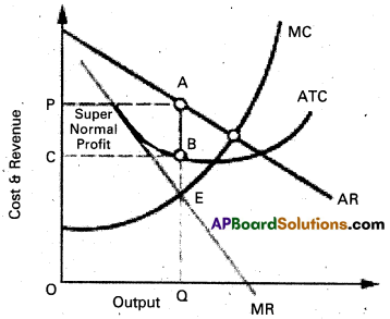
In the above diagram on ‘OX’ axis measures output and OY axis measures cost. AR is Average Revenue curve, AC is Average Cost curve. In the above diagram at E point where MC = MR at that point the monopolist determine the output. Price is determine where this output line touches the AR line. In the above diagram for producing OQ quantity cost of production is OCBQ and revenue is OPAQ.
Profit = Revenue – Cost
= PACB shaded area is profit under monopoly.

Short Answer Questions

Question 1.
What are the main features of perfect competition ?
Answer:
Perfect competitive market is one in which the number of buyers and sellers is very large, all engaged in buying and selling a homogeneous products without any restrictions.
The following are the features of perfect competition :
1) Large number of buyers and sellers : Under perfect competition the number of buyers and sellers are large. The share of each seller and buyer in total supply or total demand is small. So no buyer and seller cannot influence the price. The price is determine only demand and supply. Thus the firm is price taker.

2) Homogeneous product: The commodities produced by all the firm of an industry are homogeneous or identical. The cross elasticity of products of sellers is infinite. As a result, single price will rule in the industry.

3) Free entry and exit: In this competition there is a freedom of free entry and exit. If existing firms are getting profits. New firms enter into the market. But when a firm getting losses, it would leave to the market.

4) Perfect mobility of factors of production : Under perfect competition the factors of production are freely mobile between the firms. This is useful for free entry and exits of firms.

5) Absence of transport cost: There are no transport cost. Due to this, price of the commodity will be the same throughout the market.

6) Perfect knowledge of the economy : All the buyers and sellers have full information regarding the prevailing and future prices and availability of the commodity. Information regarding market conditions is availability of commodity.

Question 2.
What is meant by price discrimination ? Explain various methods of price discrimination.
Answer:
Price discrimination refers to the practice of a monopolist charging different prices for different customers of. the same product.
In the words of Joan Robinson “The act of selling the same article, produced under single control at different prices to different buyers is known as price discrimination”. Price discrimination is of three types. 1. Personal 2. Local 3. Use or trade discrimination.

1. Personal discrimination : When a seller charges different prices from different persons.
   Ex : A book is sold ₹ 15/- to one person and other person at discount rate of ?
2. Local discrimination : When a seller charges different prices from people of different localities or places.
   Ex : Dumping.
3. Use discrimination : When different prices of commodity are charged according to the uses to which the commodity is put is known discrimination is according to use.
   Ex : Electricity is sold at a cheaper rate for uses of domestic purposes than for industrial purposes.

Question 3.
Define Oligopoly.
Answer:
The term ‘Oligopoly’ is derived from two Greek word “Oligoi” meaning a few and “Pollein” means to sell. Oligopoly refers to a market situation in which the number of sellers dealing in a homogeneous or differentiated product is small. It is called competition among the few. The main features of oligopoly are the following.

1. Few sellers of the product.
2. There is interdependence in the determination of price.
3. Presence of monopoly power.
4. There is existence of price rigidity.
5. There is excessive selling cost or advertisement cost.

Question 4.
Compare Perfect competition and Monopoly.
Answer:
Perfect competition

1. There is large number of sellers.
2. All products are homogeneous.
3. There is freedom of free entry and exists.
4. There is difference between industry and firm.
5. Industry determines the price and firm receives the price.
6. There is universal price.
7. The AR, MR curves are parallel to ‘X, axis.

Monopoly

1. There is only one seller.
2. No close substitutes.
3. There is no freedom of free entry and exists.
4. Industry and firm both are same.
5. Firm alone determine the price.
6. Price discrimination is possible.
7. The AR, MR curves are different and slopes downs from left to right.

Additional Questions

Question 5.
Define Monopolistic competition. Explain the important characteristics of Monopolistic competition.
Answer:
It is a market with many sellers for a product but the products are different in certain respects. It is mid way of monopoly and perfect competition. Prof. E.H. Chamberlin and Mrs. Joan Robinson pioneered this market analysis.
Characteristics of Monopolistic competition :

1. Relatively small number of firms : The number of firms in this market are less than that of perfect competition. No one should not control the output in the market as a result of high competition.
2. Product differentiation : One of the features of monopolistic competition is product
   differentiation. It take the form of brand names, trade marks etc. It cross elasticity of demand is very high.
3. Entry and exit: Entry into the industry is unrestricted. New firms are able to commence production of very close substitutes for the existing brands of the product.
4. Selling cost: Advertisement or sales promotion technique is the important feature of Monopolitic competition. Such costs are called selling costs.
5. More Elastic Demand : Under this competition the demand curve slopes downwards from left to the right. It is highly elastic.

Question 6.
Explain the price determination under perfect competition ?
Answer:
Perfect competition is a competition in which the number of buyers and sellers is very large. All enged in buying and selling a homogeneous without any restrictions.

Under this competition there are large no. of by buyers and sellers no buyer is.a seller can’t influence market price all products are homogeneous there is a freedom of free entry and exit. There is a perfect mobility of factors are production. There is no transport cost these are the main features are perfect competition.

Price determination:
Under perfect competition sellers and buyers can’t decide the price industry decides the price of the good in the supply and demand determined the price these can shown in the following table.

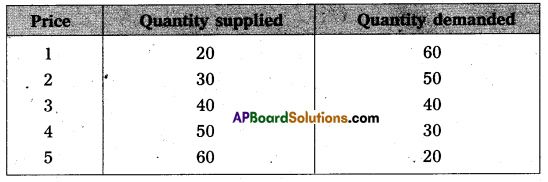
In this competition where demand supply both are equal at that point price and output determine the table changes in price always lead to a change in supply and demand as price increases there is a fall in the quantity demanded. The relation between price and demand is negative. The relation between price and supply is positive. It can be observe the table price 1 ₹ market demand 60 and supply is 20. When price increases 5 ₹ supply increases’ 60 and demand decreases 20. When the price is 3 ₹ the demand supply are equal that is 40 these price called equilibrium price. This process is explain with help of the diagram.

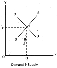
In the diagram ‘OX’ axis shown demand and supply OY’ axis represented price. DD demand curve, ‘SS’ is supply curve. In the diagram the demand curve and supply curve intersect at point E. Where the price is ‘OP’ and output is ‘OQ’.

Very Short Answer Questions

Question 1.
Market
Answer:
Market is place where commodities are brought and sold and where buyers and sellers meet. Communication facilities help us today to purchase and sell without sell without going to the market. All the activities take place is now called as market.

Question 2.
Local Market
Answer:
A product is said to have local market, when buyers and sellers of the product carry on the business in a particular locality. These goods are highly perishable cannot to take to distant places. They cannot even stored for a longer time.
Ex : Vegetables, milk, fruits etc.

Question 3.
National Market
Answer:
A National Market is said to exist when a commodity is demanded and supplies all over our country.
Ex : Rice, wheat, sugar etc. .

Question 4.
Monopoly
Answer:
Mono means single, Poly means seller. In this market single seller and there is no close substitutes. The monopolist is a price maker.

Question 5.
Monopolistic Competitions
Answer:
It is a market where several firms produce same commodity with small differences is called monopolistic competition. In this market producers to produce close substitute goods.
Ex : Soaps, cosmetics etc.

Question 6.
Oligopoly
Answer:
A market with a small number of producer is called oligopoly. The product may be homogeneous or may be differences. This market exists in automobiles, electricals etc.

Question 7.
Duopoly [march 16]
Answer:
When there are only two sellers of a product, there exist -duopoly. Each seller under duopoly must consider the other firms reactions to any changes that he make in price or output. They make decisions either independently or together.

Question 8.
Equilibrium Price
Answer:
Equilibrium price is that price where demand and supply are equal in the market.

Question 9.
Price discrimination [March 18, 17, 16]
Answer:
Monopolist will charge different prices for the same commodity or service in the market. This is known as discriminating monopoly or price discrimination.

Question 10.
Selling Costs [March 18, 17]
Answer:
An important feature of monopolistic market is every firm makes expenditure to sell more output. Advertisements through newspapers, journals, electronic media etc., these methods are used to attract more consumers by each firm.

Additional Question

Question 11.
Perfect competition
Answer:
In this market large number of buyers and sellers who promote competition. In this market goods are homogeneous. There is no transport fares and publicity costs. So price is uniform of any market.